
Update (2025-07-10): Minor edits to compute cumulative power by analysis and correct table numbering. Render with gsDesign2 1.1.5 and simtrial 1.0.0.
Update (2025-06-27): The way to specify weights for WLR designs has changed to match the new syntax in gsDesign2 1.1.4, which is now used to render this post.
Overview
We consider asymptotic approximations and corresponding simulations for group sequential designs with delayed treatment effects. We demonstrate:
- the importance of both adequate events and adequate follow-up duration to ensure power in a fixed design, and
- the importance of guaranteeing a reasonable amount of \(\alpha\)-spending for the final analysis in a group sequential design.
We demonstrate the concept of spending time as an effective way to adapt. Traditionally Lan and DeMets (1983), spending has been done according to targeting a specific number of events for an outcome at the end of the trial. However, for delayed treatment effect scenarios there is substantial literature (e.g., Lin et al. 2020; Roychoudhury et al. 2021) documenting the importance of adequate follow-up duration in addition to requiring an adequate number of events under the traditional proportional hazards assumption.
While other approaches could be taken, we have found the spending time approach generalizes well for addressing a variety of scenarios. The fact that spending does not need to correspond to information fraction was perhaps first raised by Lan and DeMets (1989) where calendar-time spending was discussed. However, we note that Michael A. Proschan, Lan, and Wittes (2006) have raised other scenarios where spending alternatives are considered. These approaches are generally more complicated to implement than the spending time approach suggested here. Two specific spending alternative approaches are examined here:
- Spending according to the minimum of planned and observed event counts. This is suggested for the delayed effect examples.
- Spending fixed amounts at analyses as suggested by Fleming, Harrington, and O’Brien (1984).
Regardless of the spending approach, it is important that timing of analyses be pre-defined in a way that is independent of observed treatment effect. This independence assumption is required to use the usual asymptotic normal calculations for computing group sequential boundary crossing probabilities. As noted by Michael A. Proschan, Follmann, and Waclawiw (1992), issues arising due to nefarious strategies when treatment differences are known at interim analysis can be largely limited by appropriate approaches. We revisit these for the \(\alpha\)-spending approach that we extend here and the fixed interim \(\alpha\)-spending method of Fleming, Harrington, and O’Brien (1984). Asymptotic distribution theory is always determined by statistical information at analyses that information is proportional to event counts for the logrank test. However, spending only needs to increase with event counts and there is no requirement that spending be a direct function of event count. While spending will always be an implicit or indirect function of event count, the function can be much easier to express by using the concept of spending time as in the cases noted above.
Computing preliminaries
Attach packages.
library(gsDesign)
library(gsDesign2)
library(tibble)
library(dplyr)
library(gt)
library(ggplot2)
library(parallelly)
library(doFuture)
library(purrr)
library(DT)
library(simtrial)
library(tictoc)
library(cowplot)
# Set to TRUE if large simulations are to be run and saved.
# Set to FALSE if simulations have already been run and saved and you want to load them.
run_simulations <- TRUESet up parallel computing.
cores_used <- 32
message("Parallelizing across ", cores_used, " CPUs")

# Set up the future plan to use the specified number of parallel workers
plan("multisession", workers = cores_used)
Set seed and number of simulations.
# Set a seed for reproducibility and use `.options.future = list(seed = TRUE)`
# for parallel-safe RNG. Use foreach + %dofuture% to perform parallel computation.
set.seed(42)
nsim <- 100000
Design assumptions
We begin with assumptions for the group sequential design as well as for alternate scenarios. The approach taken for the asymptotic normal approximation for the logrank test uses an average hazard ratio approach for approximating treatment effect (Mukhopadhyay et al. (2020)). When group sequential analyses are performed, we justify the joint distribution of logrank tests by the theory of Tsiatis (1982). Simulations are easily run for each scenario to verify asymptotic approximations of operating characteristics.
# Only one enrollment assumption used
# This could be important to vary
enrollRates <- define_enroll_rate(duration = 12, rate = 1)
# Planned study duration
analysisTimes <- 36
# Constant dropout rate across all scenarios
dropoutRate <- 0.001
# 1-sided Type I error
alpha <- 0.025
# Targeted Type II error (1 - power) for original plan (scenario 1)
beta <- 0.1
scenarios <- tribble(
  ~i, ~ControlMedian, ~Delay, ~hr1, ~hr2,              ~Scenario,
   1,             12,      4,    1,  0.6,        "Original plan",
   2,             10,      6,  1.2,  0.5, "Events accrue faster",
   3,             16,      6,    1, 0.55, "Events accrue slower",
   4,             12,      4,  0.7,  0.7, "Proportional hazards",
   5,             12,      4,    1,    1,      "Null hypothesis"
)
We consider 5 failure rate scenarios for group sequential design.
Control observations are always exponential with a scenario-specific failure rate.
Experimental observations are piecewise exponential with a hazard ratio hr1
for duration Delay (Delay) and hazard ratio hr2 thereafter.
scenarios |>
  transmute(
    Scenario = factor(Scenario),
    "Control Median" = factor(ControlMedian),
    Delay = factor(Delay),
    hr1 = factor(hr1),
    hr2 = factor(hr2)
  ) |>
  datatable(
    options = list(
      pageLength = 5,
      autoWidth = TRUE,
      columnDefs = list(list(className = "dt-center", targets = "_all"))
    ),
    filter = "top",
    caption = "Table 1: Failure rate scenarios studied"
  )
Fixed design
# Fixed design, single stratum
# Find sample size for 36 month trial under given
# enrollment and sample size assumptions
failRates <- define_fail_rate(
  duration = c(scenarios$Delay[1], 100),
  fail_rate = log(2) / scenarios$ControlMedian[1],
  hr = c(scenarios$hr1[1], scenarios$hr2[1]),
  dropout_rate = dropoutRate
)

xx <- gs_design_ahr(
  enroll_rate = enrollRates,
  fail_rate = failRates,
  alpha = alpha,
  beta = beta,
  info_frac = NULL,
  analysis_time = analysisTimes,
  ratio = 1,
  binding = FALSE,
  upper = gs_b,
  upar = qnorm(0.975),
  lower = gs_b,
  lpar = qnorm(0.975),
  h1_spending = TRUE,
  test_upper = TRUE,
  test_lower = TRUE,
) |> to_integer()

Events <- xx$analysis$event
N <- xx$analysis$n
enrollRates$rate <- N / enrollRates$duration
upar <- qnorm(0.975)
lpar <- upar
output <- NULL
for (i in 1:nrow(scenarios)) {
# Set failure rates
# Failure rates from 1st scenario for design
failRates <- define_fail_rate(
duration = c(scenarios$Delay[i], 100),
fail_rate = log(2) / scenarios$ControlMedian[i],
hr = c(scenarios$hr1[i], scenarios$hr2[i]),
dropout_rate = dropoutRate
)
# Require events only
yEvents <- gs_power_ahr(
enroll_rate = enrollRates,
fail_rate = failRates,
event = Events,
analysis_time = NULL,
upar = upar,
upper = gs_b,
lpar = lpar,
lower = gs_b
)
# Require time only
yTime <- gs_power_ahr(
enroll_rate = enrollRates,
fail_rate = failRates,
event = NULL,
analysis_time = analysisTimes,
upar = upar,
upper = gs_b,
lpar = lpar,
lower = gs_b
)
# Require events and time for analysis timing
yBoth <- gs_power_ahr(
enroll_rate = enrollRates,
fail_rate = failRates,
event = Events,
analysis_time = analysisTimes,
upar = upar,
upper = gs_b,
lpar = lpar,
lower = gs_b
)
output <- rbind(
output,
tibble(
i = i,
Scenario = scenarios$Scenario[i],
"Control Median" = scenarios$ControlMedian[i],
Delay = scenarios$Delay[i],
HR1 = scenarios$hr1[i],
HR2 = scenarios$hr2[i],
Timing = "Event-based",
N = N,
Events = yEvents$analysis$event,
Time = yEvents$analysis$time,
AHR = yEvents$analysis$ahr,
Power = yEvents$bound$probability[1],
`HR at bound` = yEvents$bound$`~hr at bound`[1]
),
tibble(
i = i,
Scenario = scenarios$Scenario[i],
"Control Median" = scenarios$ControlMedian[i],
Delay = scenarios$Delay[i],
HR1 = scenarios$hr1[i],
HR2 = scenarios$hr2[i],
Timing = "Time-based",
N = N,
Events = yTime$analysis$event,
Time = yTime$analysis$time,
AHR = yTime$analysis$ahr,
Power = yTime$bound$probability[1],
`HR at bound` = yTime$bound$`~hr at bound`[1]
),
tibble(
i = i,
Scenario = scenarios$Scenario[i],
"Control Median" = scenarios$ControlMedian[i],
Delay = scenarios$Delay[i],
HR1 = scenarios$hr1[i],
HR2 = scenarios$hr2[i],
Timing = "Max of time- and event-cutoff",
N = N,
Events = yBoth$analysis$event,
Time = yBoth$analysis$time,
AHR = yBoth$analysis$ahr,
Power = yBoth$bound$probability[1],
`HR at bound` = yBoth$bound$`~hr at bound`[1]
)
)
}A sample size of 422 and 312 targeted events was derived based on Scenario 1 assumptions using the method of Zhao, Zhang, and Anderson (2024). This method computes an average hazard ratio at the time of analysis that approximates what is produced by a Cox regression model. We will verify this below using simulated trials. The design has the following additional characteristics:
- An exponential dropout rate of 0.001 in both treatment groups.
- A constant random enrollment rate is planned for 12 months; piecewise constant enrollment is also an option in the software.
- Sample size rounded up to an even number.
- Targeted events rounded up to an integer.
- Planned analysis time at 36 months.
- Spending is based on the information fraction at the planned analysis times using a Lan-DeMets spending function to approximate the O’Brien-Fleming spending function.
- One-sided testing only; no futility bound.
- Sample size rounded to an even number, event counts rounded to the nearest integer for interim analyses and rounded up for the final analysis.
Table 2 summarizes operating characteristics for the 3 scenarios with each of the analysis timing methods. For event-based timing, the second scenario is more poorly powered than for calendar-based timing. For calendar-based timing, the third scenario is more poorly powered than for event-based timing. Thus, requiring both calendar duration and the targeted number of events before performing analysis ensures good power for all 3 scenarios; neither calendar- nor event-based timing achieve this goal. We note a few things about the alternate strategies:
- The approximate hazard ratio required for statistical significance is close to 0.8 for all scenarios. Thus, if this is used as one measure of clinical significance, we have not gamed the timing of the final analysis to reach significance with a substantially lesser treatment effect.
- For the scenario with more events accruing early and a longer effect delay, the increased events (380 vs 342) and bigger underlying treatment effect (AHR of 0.78 vs 0.76) achieved by delaying the analysis time resulted in a meaningful power increase (64% to 77%),
- For the scenario with slower event accrual, delaying the analysis until the targeted events accrue compared to analyzing at the targeted time resulted in a larger number of expected events (342 vs. 295), more substantial average hazard reduction (0.715 vs 0.735) and greater power (87% vs 75%).
Since trials represent a very large investment of patients, provider efforts (care and follow-up), and money, the gains from setting timing based on the maximum of event- and calendar-targets has important benefits. While this strategy can result in a delay in study completion, we can still do group sequential analysis to stop early for a larger than a conservatively planned treatment effect used for design.
output |>
  select(-i) |>
  group_by(Timing) |>
  gt() |>
  fmt_number(columns = c(Events, Time), decimals = 1) |>
  fmt_number(columns = c(AHR, Power, "HR at bound"), decimals = 3) |>
  tab_header("Table 2: Asymptotic approximations of design operating characteristics",
    subtitle = "Evaluating final analysis timing"
)| Table 2: Asymptotic approximations of design operating characteristics | ||||||||||
| Evaluating final analysis timing | ||||||||||
| Scenario | Control Median | Delay | HR1 | HR2 | N | Events | Time | AHR | Power | HR at bound |
|---|---|---|---|---|---|---|---|---|---|---|
| Event-based | ||||||||||
| Original plan | 12 | 4 | 1.0 | 0.60 | 422 | 312.0 | 36.0 | 0.692 | 0.901 | 0.801 |
| Events accrue faster | 10 | 6 | 1.2 | 0.50 | 422 | 312.0 | 30.6 | 0.771 | 0.630 | 0.801 |
| Events accrue slower | 16 | 6 | 1.0 | 0.55 | 422 | 312.0 | 47.5 | 0.661 | 0.953 | 0.801 |
| Proportional hazards | 12 | 4 | 0.7 | 0.70 | 422 | 312.0 | 35.0 | 0.700 | 0.882 | 0.801 |
| Null hypothesis | 12 | 4 | 1.0 | 1.00 | 422 | 312.0 | 30.1 | 1.000 | 0.025 | 0.801 |
| Time-based | ||||||||||
| Original plan | 12 | 4 | 1.0 | 0.60 | 422 | 312.0 | 36.0 | 0.692 | 0.901 | 0.801 |
| Events accrue faster | 10 | 6 | 1.2 | 0.50 | 422 | 335.5 | 36.0 | 0.748 | 0.755 | 0.807 |
| Events accrue slower | 16 | 6 | 1.0 | 0.55 | 422 | 268.5 | 36.0 | 0.682 | 0.878 | 0.787 |
| Proportional hazards | 12 | 4 | 0.7 | 0.70 | 422 | 317.0 | 36.0 | 0.700 | 0.887 | 0.802 |
| Null hypothesis | 12 | 4 | 1.0 | 1.00 | 422 | 342.2 | 36.0 | 1.000 | 0.025 | 0.809 |
| Max of time- and event-cutoff | ||||||||||
| Original plan | 12 | 4 | 1.0 | 0.60 | 422 | 312.0 | 36.0 | 0.692 | 0.901 | 0.801 |
| Events accrue faster | 10 | 6 | 1.2 | 0.50 | 422 | 335.5 | 36.0 | 0.748 | 0.755 | 0.807 |
| Events accrue slower | 16 | 6 | 1.0 | 0.55 | 422 | 312.0 | 47.5 | 0.661 | 0.953 | 0.801 |
| Proportional hazards | 12 | 4 | 0.7 | 0.70 | 422 | 317.0 | 36.0 | 0.700 | 0.887 | 0.802 |
| Null hypothesis | 12 | 4 | 1.0 | 1.00 | 422 | 342.2 | 36.0 | 1.000 | 0.025 | 0.809 |
Simulation of fixed design
We use simulation to verify the power approximations above as well as whether
Type I error is controlled at the targeted one-sided 2.5%.
Table 3 shows that with \(10^{5}\) simulated trials, the computations from Table 2
provide good approximations.
The SE(Power) provides the standard error for the simulation power approximation
for each scenario as a measure of accuracy.
The average in the HR column is the geometric average of the Cox regression
estimate of the hazard ratio.
if (run_simulations) {
  sim_summary <- NULL
  tic(paste("Fixed design simulation duration for", nsim, "simulated trials"))
  for (i in seq_along(scenarios$i)) {
    # Get failure rate and event rate assumptions from scenario i = 1
    rates <- define_fail_rate(
      duration = c(scenarios$Delay[i], 100),
      fail_rate = log(2) / scenarios$ControlMedian[i],
      hr = c(scenarios$hr1[i], scenarios$hr2[i]),
      dropout_rate = dropoutRate
    )
    # Run a simulation for power
    sim <- sim_fixed_n(
      n_sim = nsim,
      enroll_rate = xx$enroll_rate,
      sample_size = max(xx$analysis$n),
      target_event = max(xx$analysis$event),
      total_duration = max(xx$analysis$time),
      fail_rate = rates
    )

    # Summarize results
    sim_summary <- rbind(
      sim_summary,
      sim |> select(-names(sim)[1:4]) |> group_by(cut) |>
        summarise(
          Scenario = scenarios$Scenario[i], Simulations = nsim,
          Power = mean(z >= qnorm(0.975)),
          "SE(Power)" = sd(z >= qnorm(0.975)) / sqrt(nsim),
          HR = exp(mean(ln_hr)), "E(Duration)" = mean(duration),
          "SD(Duration)" = sd(duration), "E(Events)" = mean(event),
          "SD(Events)" = sd(event)
        )
    )
  }
  save(sim_summary, file = "FixedDesignSimulation.RData")
  toc()
} else {
  load("FixedDesignSimulation.RData")
}
#> Fixed design simulation duration for 1e+05 simulated trials: 830.2 sec elapsedsim_summary |>
transmute(
Scenario = factor(Scenario),
Cut = factor(cut),
Power = round(Power, 4),
"SE(Power)" = round(`SE(Power)`, 4),
HR = round(HR, 3),
"E(Duration)" = round(`E(Duration)`, 1),
"SD(Duration)" = round(`SD(Duration)`, 1),
"E(Events)" = round(`E(Events)`, 1),
"SD(Events)" = round(`SD(Events)`, 1)
) |>
group_by(Cut) |>
datatable(
options = list(
pageLength = 5,
autoWidth = TRUE,
columnDefs = list(list(className = "dt-center", targets = "_all"))
),
filter = "top",
caption = "Table 3: Simulation results by scenario and data cutoff method"
)# gt() |>
# fmt_number(columns = c(HR, "Power", "SE(Power)"), decimals = 3) |>
# fmt_number(columns = c("E(Duration)", "SD(Duration)", "E(Events)", "SD(Events)"), decimals = 1) |>
# tab_header(title = "Table 3: Simulation results by scenario and data cutoff method")Simulations were performed with the simtrial::sim_fixed_n() function using
parallel computing with 32 CPUs. While the user sets up the
number of CPU cores used and parallel backend, the parallel computing is
otherwise implemented automatically by simtrial::sim_fixed_n().
Group sequential design
Now we derive the planned design with the Original plan assumptions above. The design has the following additional characteristics. Other than the group sequential assumptions, these are the same as for the fixed design above.
- An exponential dropout rate of 0.001 in both treatment groups.
- A constant random enrollment rate is planned for 12 months; piecewise constant enrollment is also an option in the software.
- Planned analysis times at 20, 28, and 36 months.
- Spending is based on the information fraction at the planned analysis times using a Lan-DeMets spending function to approximate the O’Brien-Fleming spending function.
- One-sided testing only; no futility bound.
- Sample size rounded to an even number, event counts rounded to the nearest integer for interim analyses and rounded up for the final analysis.
# Failure rates from 1st scenario for design
failRates <- define_fail_rate(
  duration = c(scenarios$Delay[1], 100),
  fail_rate = log(2) / scenarios$ControlMedian[1],
  hr = c(scenarios$hr1[1], scenarios$hr2[1]),
  dropout_rate = dropoutRate
)
upar_design <- list(sf = gsDesign::sfLDOF, total_spend = alpha)
# Find sample size for 36 month trial under given
# enrollment and sample size assumptions
# Interim at planned information fraction
xx <- gs_design_ahr(
  enroll_rate = enrollRates,
  fail_rate = failRates,
  analysis_time = c(20, 28, 36),
  # analysisTimes,
  info_frac = NULL,
  # planned_IF,
  upper = gs_spending_bound,
  upar = upar_design,
  lpar = rep(-Inf, 3),
  lower = gs_b,
  test_lower = FALSE,
  beta = beta,
  alpha = alpha
) |> to_integer()
The planned analyses and bounds are in the table below. In spite of two interim analyses with 0.66 and 0.86 of the final planned observations, the O’Brien-Fleming spending approach preserves enough \(\alpha\) for the final analysis to be tested at a nominal 0.0201 level. While the 0.86 information fraction at the final interim may seem high, the intent to do analyses every 8 months starting at month 20 dictates this. At the final analysis, a hazard ratio of approximately 0.79 or smaller is required for a positive finding. Under the alternate hypothesis, there is a substantial probability of crossing an efficacy bound prior to the final analysis as indicated by the cumulative power of 0.35 at the first interim analysis and 0.75 at the second. We see that the expected geometric mean of the observed hazard ratio (AHR) decreases from 0.74 at the first interim to 0.71 at the second, and 0.69 at the final analysis. Thus, the longer the trial continues, the stronger the expected treatment effect is. We will see that continuing the trial long enough for the expected treatment effect to be strong is important in the scenarios that follow.
xx |>
  summary() |>
  as_gt(
    title = "Group sequential design based on original assumptions",
    subtitle = "Table 4: Delayed effect for 4 months, HR = 0.6 thereafter"
)| Group sequential design based on original assumptions | |||||
| Table 4: Delayed effect for 4 months, HR = 0.6 thereafter | |||||
| Bound | Z | Nominal p1 | ~HR at bound2 |
Cumulative boundary crossing probability
|
|
|---|---|---|---|---|---|
| Alternate hypothesis | Null hypothesis | ||||
| Analysis: 1 Time: 19.9 N: 430 Events: 209 AHR: 0.74 Information fraction: 0.66 | |||||
| Efficacy | 2.53 | 0.0057 | 0.7046 | 0.3454 | 0.0057 |
| Analysis: 2 Time: 27.9 N: 430 Events: 273 AHR: 0.71 Information fraction: 0.86 | |||||
| Efficacy | 2.20 | 0.0138 | 0.7661 | 0.7453 | 0.0156 |
| Analysis: 3 Time: 36 N: 430 Events: 318 AHR: 0.69 Information fraction: 1 | |||||
| Efficacy | 2.05 | 0.0201 | 0.7944 | 0.9009 | 0.0250 |
| 1 One-sided p-value for experimental vs control treatment. Value < 0.5 favors experimental, > 0.5 favors control. | |||||
| 2 Approximate hazard ratio to cross bound. | |||||
Same design with weighted logrank
We consider the same sample size and analysis timing but using the modestly weighted logrank (MWLR) test of Magirr and Burman (2019). Weights increase from 1 at time 0 to a maximum of 2 at the combined treatment group median and beyond. We see that power is higher than for the unweighted logrank above. Note that due to the higher weighting of later failures, the information fraction is lower for interim analyses than when using the logrank test above. Thus, the increased power relative to the logrank test above is due both to the weighting and spending changes.
gs_arm <- gs_create_arm(xx$enroll_rate, xx$fail_rate, xx$ratio)
mb_design <- gs_power_wlr(
  enroll_rate = xx$enroll_rate,
  fail_rate = xx$fail_rate,
  analysis_time = xx$analysis$time,
  # Magirr-Burman weighting for MWLR
  weight = list(method = "mb", param = list(tau = NULL, w_max = 2)),
  upper = gs_spending_bound,
  upar = upar_design,
  lpar = rep(-Inf, 3),
  lower = gs_b,
  test_lower = FALSE
) |> to_integer()
mb_design |>
summary() |>
as_gt(
title = "Group sequential design based on original assumptions",
subtitle = "Table 5: Testing with MWLR using maximum weight of 2"
)| Group sequential design based on original assumptions | |||||
| Table 5: Testing with MWLR using maximum weight of 2 | |||||
| Bound | Z | Nominal p1 | ~wHR at bound2 |
Cumulative boundary crossing probability
|
|
|---|---|---|---|---|---|
| Alternate hypothesis | Null hypothesis | ||||
| Analysis: 1 Time: 19.9 N: 430 Events: 209 AHR: 0.72 Information fraction: 0.493 | |||||
| Efficacy | 2.99 | 0.0014 | 0.6615 | 0.2725 | 0.0014 |
| Analysis: 2 Time: 27.9 N: 430 Events: 273 AHR: 0.68 Information fraction: 0.783 | |||||
| Efficacy | 2.29 | 0.0109 | 0.7577 | 0.8043 | 0.0114 |
| Analysis: 3 Time: 36 N: 430 Events: 318 AHR: 0.66 Information fraction: 13 | |||||
| Efficacy | 2.02 | 0.0215 | 0.7970 | 0.9492 | 0.0250 |
| 1 One-sided p-value for experimental vs control treatment. Value < 0.5 favors experimental, > 0.5 favors control. | |||||
| 2 Approximate hazard ratio to cross bound. | |||||
| 3 wAHR is the weighted AHR. | |||||
We check that the cumulative \(\alpha\)-spending at each analysis is as expected:
sfLDOF(alpha = 0.025, t = mb_design$analysis$info_frac0)$spend#> [1] 0.001409526 0.011392119 0.025000000Accumulation of events and average treatment effect over time
In addition to the different failure rate scenarios, we consider 3 enrollment scenarios to achieve the targeted sample size:
- The original design assumptions.
- A rate 50% higher than the original design, with 4 months less time for the expected sample size to reach the target.
- A rate 25% lower than the original design with 4 months more time for the expected sample size to reach the target.
enroll_rate_scenarios <- rbind(
  define_enroll_rate(duration = 12, rate = xx$enroll_rate$rate[1]) |>
    mutate(Enrollment = "Original"),
  define_enroll_rate(duration = 8, rate = 1.5 * xx$enroll_rate$rate[1]) |>
    mutate(Enrollment = "Faster"),
  define_enroll_rate(duration = 16, rate = 0.75 * xx$enroll_rate$rate[1]) |>
    mutate(Enrollment = "Slower")
)
enroll_rate_scenarios |>
  select(-stratum) |>
  gt() |>
  tab_header(title = "Table 6: Enrollment rate scenarios") |>
  fmt_number(columns = "rate", decimals = 1) |>
  cols_label(
    duration = "Target duration (months)", rate = "Enrollment rate per month",
    Enrollment = "Scenario"
)| Table 6: Enrollment rate scenarios | ||
| Target duration (months) | Enrollment rate per month | Scenario |
|---|---|---|
| 12 | 35.8 | Original |
| 8 | 53.7 | Faster |
| 16 | 26.9 | Slower |
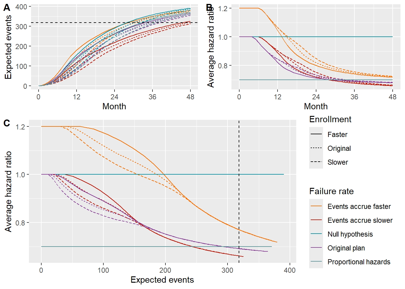
Now we compute expected events and average hazard ratio over time for each enrollment and event rate scenario. We see that for the higher event rate scenario events may accrue closer to 30 months rather than the planned 36 months (Figures A and C). For faster enrollment rates, the delayed effect as evidenced by average hazard ratio (AHR) is exaggerated (Figures B and C). The average hazard ratio appears to have an important decrease (improvement) still between 30 and 36 months (Figure B), suggesting it could be advantageous to have the trial continue for at least 36 months. For lower than planned event rates, it appears important to extend the trial past 36 months to accrue the targeted events.
output <- NULL
for (i in 1:nrow(scenarios)) {
  # Set failure rates
  failRates <- define_fail_rate(
    duration = c(scenarios$Delay[i], 100),
    fail_rate = log(2) / scenarios$ControlMedian[i],
    hr = c(scenarios$hr1[i], scenarios$hr2[i]),
    dropout_rate = dropoutRate
  )
  for (j in 1:nrow(enroll_rate_scenarios)) {
    # Find sample size for 30 month trial under given
    # enrollment and sample size assumptions
    yy <- ahr(
      enroll_rate = enroll_rate_scenarios[j, ],
      fail_rate = failRates,
      total_duration = c(0.001, 1:48),
      ratio = 1
    ) |>
      mutate(
        Enrollment = enroll_rate_scenarios$Enrollment[j],
        Scenario = scenarios$Scenario[i]
      )
    output <- rbind(output, yy)
  }
}
p1 <- output |> ggplot(aes(x = time, y = event, color = Scenario, lty = Enrollment)) +
geom_line() +
geom_hline(yintercept = max(xx$analysis$event), linetype = "dashed") +
scale_x_continuous(breaks = seq(0, 48, 12)) +
guides(lty = "none", color = "none") +
ggsci::scale_color_futurama() +
ylab("Expected events") +
xlab("Month")
p2 <- output |> ggplot(aes(x = time, y = ahr, color = Scenario, lty = Enrollment)) +
geom_line() +
scale_x_continuous(breaks = seq(0, 48, 12)) +
guides(lty = "none", color = "none") +
ggsci::scale_color_futurama() +
ylab("Average hazard ratio") +
xlab("Month")
p3 <- output |> ggplot(aes(x = event, y = ahr, color = Scenario, lty = Enrollment)) +
geom_line() +
geom_vline(xintercept = max(xx$analysis$event), linetype = "dashed") +
ggsci::scale_color_futurama() +
guides(color = guide_legend(title = "Failure rate")) +
ylab("Average hazard ratio") +
xlab("Expected events") +
theme(legend.position = "right")top_row <- cowplot::plot_grid(p1, p2, labels = c("A", "B"), label_size = 12)
cowplot::plot_grid(top_row, p3,
labels = c("", "C"), label_size = 12, ncol = 1,
rel_heights = c(0.4, 0.6)
)
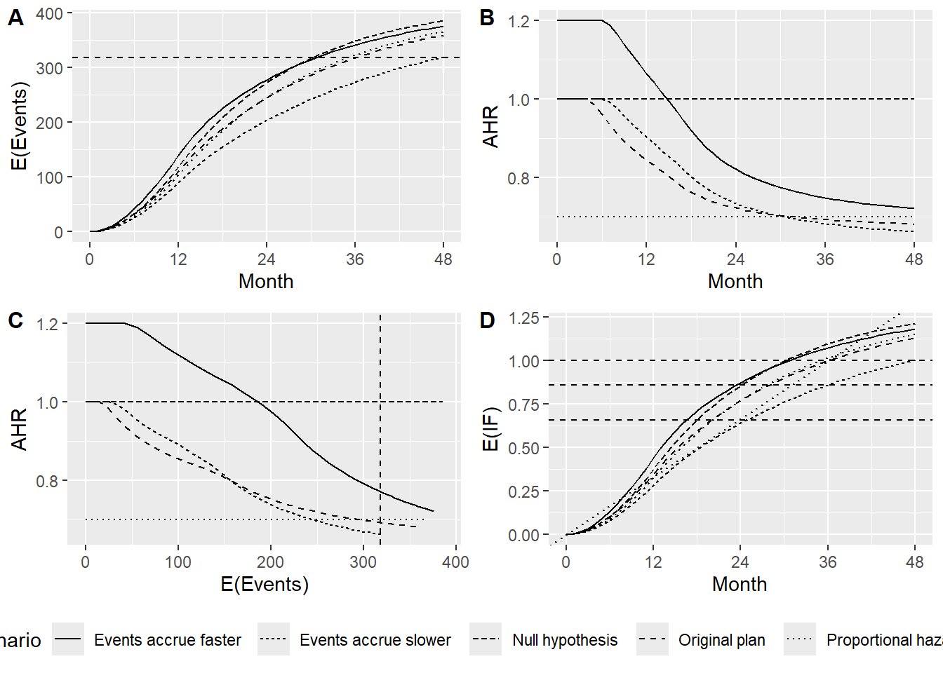
To simplify the above plots without losing the basic interpretation, we consider the different failure rate scenarios only for the original enrollment rate scenario. We add a plot of the expected information fraction for the scenarios above using the planned maximum information fraction from the original design as the denominator.
p1 <- output |>
  filter(Enrollment == "Original") |>
  ggplot(aes(x = time, y = event, lty = Scenario)) +
  geom_line() +
  geom_hline(yintercept = max(xx$analysis$event), linetype = "dashed") +
  scale_x_continuous(breaks = seq(0, 48, 12)) +
  guides(lty = "none", color = "none") +
  ggsci::scale_color_futurama() +
  ylab("E(Events)") +
  xlab("Month")

p2 <- output |>
  filter(Enrollment == "Original") |>
  ggplot(aes(x = time, y = ahr, lty = Scenario)) +
  geom_line() +
  scale_x_continuous(breaks = seq(0, 48, 12)) +
  guides(lty = "none", color = "none") +
  ggsci::scale_color_futurama() +
  ylab("AHR") +
  xlab("Month")

p3 <- output |>
  filter(Enrollment == "Original") |>
  ggplot(aes(x = event, y = ahr, lty = Scenario)) +
  geom_line() +
  geom_vline(xintercept = max(xx$analysis$event), linetype = "dashed") +
  ggsci::scale_color_futurama() +
  guides(lty = "none") +
  ylab("AHR") +
  xlab("E(Events)") +
  theme(legend.position = "right")

p4 <- output |>
  filter(Enrollment == "Original") |>
  mutate(IF = info0 / max(xx$analysis$info0)) |>
  ggplot(aes(x = time, y = IF, lty = Scenario)) +
  geom_line() +
  scale_x_continuous(breaks = seq(0, 48, 12)) +
  ggsci::scale_color_futurama() +
  ylab("E(IF)") +
  xlab("Month") +
  geom_hline(yintercept = 1, linetype = "dashed") +
  geom_hline(yintercept = xx$analysis$info_frac0[2], linetype = "dashed") +
  geom_hline(yintercept = xx$analysis$info_frac0[1], linetype = "dashed") +
  geom_abline(intercept = 0, slope = 1 / max(xx$analysis$time), linetype = "dotted") +
  theme(legend.position = "bottom")

legend <- get_legend(p4)
p4a <- p4 + theme(legend.position = "none")
#  guides(lty = "none", color = "none")

# Now put all of these plots in a grid
top_row <- cowplot::plot_grid(
  p1, p2, p3, p4a,
  labels = c("A", "B", "C", "D"),
  label_size = 12,
  ncol = 2,
  rel_heights = c(0.5, 0.5)
)
cowplot::plot_grid(
  top_row, legend,
  labels = c("", ""),
  label_size = 12,
  ncol = 1,
  rel_heights = c(0.9, 0.1)
)
Alternate analysis timing and \(\alpha\)-spending strategies
Timing of analyses and \(\alpha\)-spending are done 3 ways:
- Event-based timing and spending based on planned events above.
- Time-based analyses and spending based on planned calendar time and planned spending above.
- Analyses at maximum of time when targeted events and targeted calendar time are reached, spending as minimum of planned and actual.
Another approach that might be considered is to analyze after, say, every 8 months until the targeted events are reached with the first interim analysis at 20 months; this has not been undertaken here as the 3rd approach above is presumed adequate to demonstrate the principle we are suggesting.
We will focus on examples with the planned enrollment rates as these are adequate for demonstrating the issues we are considering. You can see in the plot above that different enrollment rates can impact time to achieve targeted events which may be particularly challenging for the calendar-based spending approach.
# Planned enrollment rates from design
enrollRates <- xx$enroll_rate
# Planned information fraction at interim(s) and final
planned_IF <- xx$analysis$event / max(xx$analysis$event)
# Spending time entered in timing for planned spending
upar_planned_spending <- list(sf = gsDesign::sfLDOF, total_spend = alpha, timing = planned_IF)
# Information fraction (event-based) spending
max_info0 <- max(xx$analysis$info0)
upar_IF_spending <- list(
  sf = gsDesign::sfLDOF,
  total_spend = alpha,
  param = NULL,
  timing = NULL,
  max(max_info = xx$analysis$info0)
)
# Lower spending
lpar <- rep(-Inf, 2)
# Events for event-based analysis timing
Events <- xx$analysis$event
# Planned analysis times
analysisTimes <- xx$analysis$time
The following table displays the results.
output <- NULL
for (i in 1:nrow(scenarios)) {
  # Set failure rates
  # Failure rates from 1st scenario for design
  failRates <- define_fail_rate(
    duration = c(scenarios$Delay[i], 100),
    fail_rate = log(2) / scenarios$ControlMedian[i],
    hr = c(scenarios$hr1[i], scenarios$hr2[i]),
    dropout_rate = dropoutRate
  )
  # Event-based timing and spending
  yIF <- gs_power_ahr(
    enroll_rate = enrollRates,
    fail_rate = failRates,
    event = Events,
    analysis_time = NULL,
    upper = gs_spending_bound,
    upar = upar_IF_spending,
    lower = gs_b,
    lpar = rep(-Inf, length(Events))
  ) |> to_integer()
  # Interim spending based on planned IF; timing based on calendar times
  yPlanned <- gs_power_ahr(
    enroll_rate = enrollRates,
    fail_rate = failRates,
    event = NULL,
    analysis_time = analysisTimes,
    upper = gs_spending_bound,
    upar = upar_planned_spending,
    lower = gs_b,
    lpar = rep(-Inf, length(analysisTimes))
  )
  # Interim timing at max of planned time, events
  # Spending is min of planned and actual
  upar_both <- list(
    sf = gsDesign::sfLDOF, total_spend = alpha, param = NULL,
    timing = pmin(planned_IF, Events / max(Events)), max_info = NULL
  )
  yBoth <- gs_power_ahr(
    enroll_rate = enrollRates,
    fail_rate = failRates,
    event = Events,
    analysis_time = analysisTimes,
    upper = gs_spending_bound,
    upar = upar_both,
    lower = gs_b,
    lpar = rep(-Inf, length(Events))
  )

  output <- rbind(
    output,
    # Event-based spending
    tibble(
      i = i, Scenario = scenarios$Scenario[i], "Control Median" = scenarios$ControlMedian[i],
      Delay = scenarios$Delay[i], HR1 = scenarios$hr1[i], HR2 = scenarios$hr2[i],
      Spending = "IF", Analysis = yIF$analysis$analysis,
      N = yIF$analysis$n, Events = yIF$analysis$event, Time = yIF$analysis$time,
      "Nominal p" = pnorm(-yIF$bound$z),
      Power = yIF$bound$probability, AHR = yIF$analysis$ahr,
      `HR at bound` = yIF$bound$`~hr at bound`, IF = yIF$analysis$info_frac0,
      "Spending time" = yIF$analysis$info_frac0
    ),
    # Planned time, event-based spending
    tibble(
      i = i, Scenario = scenarios$Scenario[i], "Control Median" = scenarios$ControlMedian[i],
      Delay = scenarios$Delay[i], HR1 = scenarios$hr1[i], HR2 = scenarios$hr2[i],
      Spending = "Planned", Analysis = yPlanned$analysis$analysis,
      N = yPlanned$analysis$n, Events = yPlanned$analysis$event, Time = yPlanned$analysis$time,
      "Nominal p" = pnorm(-yPlanned$bound$z),
      Power = yPlanned$bound$probability, AHR = yPlanned$analysis$ahr,
      `HR at bound` = yPlanned$bound$`~hr at bound`, IF = yPlanned$analysis$info_frac0,
      "Spending time" = upar_planned_spending$timing
    ),
    # Max of planned and actual
    tibble(
      i = i, Scenario = scenarios$Scenario[i], "Control Median" = scenarios$ControlMedian[i],
      Delay = scenarios$Delay[i], HR1 = scenarios$hr1[i], HR2 = scenarios$hr2[i],
      Spending = "min(IF, Planned)", Analysis = yBoth$analysis$analysis,
      N = yBoth$analysis$n, Events = yBoth$analysis$event, Time = yBoth$analysis$time,
      "Nominal p" = pnorm(-yBoth$bound$z),
      Power = yBoth$bound$probability, AHR = yBoth$analysis$ahr,
      `HR at bound` = yBoth$bound$`~hr at bound`, IF = yBoth$analysis$info_frac0,
      "Spending time" = pmin(yBoth$analysis$info_frac0, planned_IF)
    )
  )
}
The critical difference here is demonstrated when events accrue faster than expected due to the treatment benefit emerging later. Analysis timing is the same for both spending methods. Using information fraction spending uses up 0.0194 of 0.025 \(\alpha\) at the interim analysis rather than the planned 0.012. This means that the nominal p-value for the final test is 0.0162 as opposed to 0.0222 if the planned interim spending is used. This also results in a power increase from 63.8% with information-based spending to 68.4% when planned spending is used. Being able to preserve the largest nominal bound for the final analysis is in the general spirit of setting higher bounds at interim analysis if an early stop is to be justified.
output |>
  select(-c(i, "Control Median", Delay, HR1, HR2)) |>
  mutate(
    Spending = factor(Spending, levels = c("IF", "Planned", "min(IF, Planned)")),
    Scenario = factor(Scenario)
  ) |>
  datatable(
    options =
      list(
        filter = "top",
        pageLength = 25,
        dom = "Bfrtip",
        buttons = c("copy", "csv", "excel"),
        scrollX = TRUE,
        columnDefs = list(
          list(width = "35px", targets = c(0)), # Strategy column
          list(width = "45px", targets = c(1)), # Scenario column
          list(width = "45px", targets = c(7)) # Nominal p column
          # list(width = '30px', targets = c(2, 3, 4)),  # Control Median, Delay, HR1 columns
          # list(width = '25px', targets = c(5)),  # HR2 column
          # list(width = '35px', targets = c(7, 8, 9)),  # Power, AHR, HR at bound columns
          # list(width = '30px', targets = c(10, 11))  # IF and Spending time columns
        )
      ),
    filter = "top",
    caption = "Table 7: Design characteristics by spending strategy across scenarios"
  ) |>
  formatRound(columns = c("N", "Events", "Time"), digits = 1) |>
  # formatRound(columns = c("Nominal p"), digits = 4) |>
  formatRound(columns = c("Power", "AHR", "HR at bound", "IF", "Spending time", "Nominal p"), digits = 3) |>
  htmlwidgets::onRender("
function(el, x) {
$(el).find('table').css('font-size', '0.6em');
$(el).find('td').css('padding', '1px 1px');
$(el).find('th').css('padding', '1px 1px');
$(el).find('table').css('width', 'auto');
$(el).find('.dataTables_wrapper').css('width', 'auto');

// Adjust filter box widths to match column widths
var columnWidths = [35, 45, 30, 30, 30, 25, 45, 35, 35, 35, 30, 30];
$(el).find('input').each(function(i) {
$(this).css('width', columnWidths[i] + 'px');
});
}
")
Now we summarize design characteristics by spending strategy across scenarios. We see that using the minimum of planned and actual spending retains the highest power across scenarios (A). If events accrue more slowly than planned, the minimum of planned and actual spending adapts to longer duration (B), more events (C) and a stronger effect size (AHR) than using the planned calendar timing and spending. Using event-based (IF) spending results in lower power if events accrue faster than planned due to a lesser effect size (higher AHR) and fewer events than timing analyses at the maximum of planned and actual time. Under proportional hazards and the original delayed effect scenario, all strategies have similar power. The final analysis nominal p-value is highest for the minimum of planned and actual spending, regardless of scenario (E).
# Power plot
p1 <- output |>
  filter(Analysis == 3) |>
  ggplot(aes(x = Scenario, y = Power, fill = Spending)) +
  geom_bar(stat = "identity", position = "dodge") +
  theme(axis.text.x = element_text(angle = 45, hjust = 1)) +
  ylab("Power") +
  xlab("Scenario")

# Events plot
p2 <- output |>
  filter(Analysis == 3) |>
  ggplot(aes(x = Scenario, y = Events, fill = Spending)) +
  geom_bar(stat = "identity", position = "dodge") +
  theme(axis.text.x = element_text(angle = 45, hjust = 1)) +
  ylab("Events") +
  xlab("Scenario")

# Z-score plot
p3 <- output |>
  filter(Analysis == 3) |>
  ggplot(aes(x = Scenario, y = `HR at bound`, fill = Spending)) +
  geom_bar(stat = "identity", position = "dodge") +
  theme(axis.text.x = element_text(angle = 45, hjust = 1)) +
  ylab("HR at bound") +
  xlab("Scenario")

# Display plots with increased height
cowplot::plot_grid(p1, p2, p3, ncol = 1, labels = c("A", "B", "C"), rel_heights = c(1, 1, 1))
Simulation to verify operating characteristics
We focus on the case where events accrue faster than planned to ensure that adapting spending is not impacting Type I error as well as to confirm power with the different strategies. We write a function to simulate a trial, including cutting off for analyses with different strategies.
Simulate a single trial and perform tests
# Convert failure rates to simulation format
# Scenario 1
# rates <- to_sim_pw_surv(xx$fail_rate)
# Null hypothesis
rates <- to_sim_pw_surv(xx$fail_rate |> mutate(hr = 1))

# Simulate a trial
simulate_a_trial <- function(
    n, enroll_rate, fail_rate, dropout_rate, target_events, target_time,
    block = c(
      "control", "control",
      "experimental", "experimental"
    )) {
  cut_date_events <- rep(0, length(target_events))
  cut_date_both <- rep(0, length(target_events))
  output <- NULL
  dat <- sim_pw_surv(
    n = n, stratum = data.frame(stratum = "All", p = 1),
    enroll_rate = enroll_rate, fail_rate = fail_rate,
    dropout_rate = dropout_rate, block = block
  )

  for (k in seq_along(target_events)) {
    # Time to targeted event count
    cut_date_events[k] <- get_cut_date_by_event(dat, target_events[k])
    # Time to max of targeted event count, targeted time
    cut_date_both[k] <- max(cut_date_events[k], target_time[k])
  }
  # get unique analysis time cutoffs
  cut_times <- unique(c(cut_date_events, target_time))

  # Do analyses at targeted times
  for (k in seq_along(cut_times)) {
    # Cut data
    dat_cut <- cut_data_by_date(dat, cut_times[k])
    # Get counting process dataset to be used for both tests of interest
    counting_data <- dat_cut |> counting_process(arm = "experimental")
    # Sum total events across times at which events are observed
    Events <- sum(dat_cut$event)
    # sum(counting_data$event_total) #
    # Compute logrank test
    test <- counting_data |>
      wlr(weight = fh(rho = 0, gamma = 0), return_variance = TRUE) |>
      as.data.frame() |>
      mutate(test = "lr", Time = cut_times[k], Events = Events) |>
      select(-c(method, parameter, estimate, se))
    # Compute Magirr-Burman test
    test_mb <- counting_data |>
      wlr(weight = mb(delay = Inf, w_max = 2)) |>
      # info conversion is a GUESS to match planned design; needs checking
      as.data.frame() |>
      mutate(test = "mwlr", Time = cut_times[k], Events = Events) |>
      select(-c(method, parameter, estimate, se))
    # Add a record for each of the above tests
    output <- rbind(output, test, test_mb)
  }
  # Accumulate analyses for each cutting method
  output <-
    bind_rows(
      tibble(Cut = "Events", Time = cut_date_events),
      tibble(Cut = "Time", Time = target_time),
      tibble(Cut = "Both", Time = cut_date_both)
    ) |> left_join(output, by = "Time", relationship = "many-to-many")
  # Cutoff at max of planned time, events, spending based on min of planned, actual events
  lrboth <- output |> filter(Cut == "Both" & test == "lr")
  lrboth$Analysis <- seq_along(lrboth$Events)
  lrboth$sTime <- pmin(
    xx$analysis$event / max(xx$analysis$event),
    Events / max(xx$analysis$event)
  )
  lrboth$sTime[3] <- 1 # Full spend at final analysis
  lrboth$spend <- diff(c(0, sfLDOF(alpha = alpha, t = lrboth$sTime)$spend))
  lrboth$Bound <- gsBound1(
    theta = 0, I = lrboth$Events, a = rep(-20, 3),
    probhi = lrboth$spend, tol = 1e-06, r = 18
  )$b
  lrboth$IF <- lrboth$Events / max(xx$analysis$event)
  lrboth$"Reject H0" <- ifelse(lrboth$z >= lrboth$Bound, TRUE, FALSE)
  lrboth$Spending <- "min(planned, actual)"

  # Cutoff at max of planned time, events, spending based on events
  lrbothe <- lrboth
  lrbothe$Analysis <- seq_along(lrbothe$Events)
  lrbothe$sTime <- lrbothe$Events / max(xx$analysis$event)
  # Final total spending time should be at least 1
  lrbothe$sTime[3] <- max(1, lrbothe$sTime[3])
  lrbothe$spend <- diff(c(0, sfLDOF(alpha = alpha, t = lrbothe$sTime)$spend))
  # May be instances where final event count is reached by IA 2
  # when planned time of IA2 is reached
  if (lrbothe$sTime[2] < 1) {
    lrbothe$Bound <- gsBound1(
      theta = 0, I = lrbothe$Events, a = rep(-20, 3),
      probhi = lrbothe$spend, tol = 1e-06, r = 18
    )$b
  } else {
    lrbothe$Bound <- c(
      gsBound1(
        theta = 0, I = lrbothe$Events[1:2], a = rep(-20, 2),
        probhi = lrbothe$spend[1:2], tol = 1e-06, r = 18
      )$b,
      Inf
    )
  }
  lrbothe$IF <- lrbothe$Events / max(xx$analysis$event)
  lrbothe$"Reject H0" <- ifelse(lrbothe$z >= lrbothe$Bound, TRUE, FALSE)
  lrbothe$Spending <- "Events"

  # mwlr with min(Planned, Actual) spending
  mwlrboth <- output |> filter(Cut == "Both" & test == "mwlr")
  mwlrboth$Analysis <- seq_along(mwlrboth$Events)
  mwlrboth$sTime <- pmin(
    mwlrboth$info0 / max(mb_design$analysis$info0),
    mb_design$analysis$info_frac0
  )
  mwlrboth$sTime[3] <- max(1, mwlrboth$sTime[3]) # Full spend at final analysis
  mwlrboth$spend <- diff(c(0, sfLDOF(alpha = alpha, t = mwlrboth$sTime)$spend))
  mwlrboth$Bound <- gsBound1(
    theta = 0, I = mwlrboth$info0, a = rep(-20, 3),
    probhi = mwlrboth$spend, tol = 1e-06, r = 18
  )$b
  mwlrboth$IF <- mwlrboth$info0 / max(mb_design$analysis$info0)
  mwlrboth$"Reject H0" <- ifelse(mwlrboth$z >= mwlrboth$Bound, TRUE, FALSE)
  mwlrboth$Spending <- "min(planned, actual)"

  # Cut at max of planned time, events, spending based on info0, mwlr
  mwlrbothe <- mwlrboth
  mwlrbothe$Analysis <- seq_along(mwlrbothe$info0)
  mwlrbothe$sTime <- mwlrbothe$info0 / max(mb_design$analysis$info0)
  mwlrbothe$sTime[3] <- max(1, mwlrbothe$sTime[3]) # Full spend at final analysis
  mwlrbothe$spend <- diff(c(0, sfLDOF(alpha = alpha, t = mwlrbothe$sTime)$spend))
  # May be instances where final info0 is reached by IA 2
  # when planned time of IA2 is reached
  if (mwlrbothe$sTime[2] < 1) {
    mwlrbothe$Bound <- gsBound1(
      theta = 0, I = mwlrbothe$info0, a = rep(-20, 3),
      probhi = mwlrbothe$spend, tol = 1e-06, r = 18
    )$b
  } else {
    mwlrbothe$Bound <- c(
      gsBound1(
        theta = 0, I = mwlrbothe$info0[1:2], a = rep(-20, 2),
        probhi = mwlrbothe$spend[1:2], tol = 1e-06, r = 18
      )$b,
      Inf
    )
  }
  mwlrbothe$IF <- mwlrbothe$info0 / max(mb_design$analysis$info0)
  mwlrbothe$"Reject H0" <- ifelse(mwlrbothe$z >= mwlrbothe$Bound, TRUE, FALSE)
  mwlrbothe$Spending <- "IF"

  # Cut at targeted events, lr
  lrevents <- output |> filter(Cut == "Events" & test == "lr")
  lrevents$Analysis <- seq_along(lrevents$Events)
  lrevents$sTime <- xx$analysis$info_frac0
  lrevents$spend <- diff(c(0, xx$bound$probability0))
  lrevents$Bound <- xx$bound$z
  lrevents$IF <- xx$analysis$info_frac0
  lrevents$"Reject H0" <- ifelse(lrevents$z >= lrevents$Bound, TRUE, FALSE)
  lrevents$Spending <- "Events"

  # Cut at targeted events, mwlr
  mwlrevents <- output |> filter(Cut == "Events" & test == "mwlr")
  mwlrevents$Analysis <- seq_along(mwlrevents$Events)
  mwlrevents$sTime <- mwlrevents$info0 / max(mb_design$analysis$info0)
  mwlrevents$sTime[3] <- max(1, mwlrevents$sTime[3])
  mwlrevents$spend <- diff(c(0, sfLDOF(alpha = alpha, t = mwlrevents$sTime)$spend))
  mwlrevents$Bound <- gsBound1(
    theta = 0, I = mwlrevents$info0, a = rep(-20, 3),
    probhi = mwlrevents$spend, tol = 1e-06, r = 18
  )$b
  mwlrevents$IF <- mwlrevents$info0 / max(mb_design$analysis$info0)
  mwlrevents$"Reject H0" <- ifelse(mwlrevents$z >= mwlrevents$Bound, TRUE, FALSE)
  mwlrevents$Spending <- "IF"

  # Cut at targeted time, lr
  lrtime <- output |> filter(Cut == "Time" & test == "lr")
  lrtime$Analysis <- seq_along(lrtime$Events)
  lrtime$sTime <- xx$analysis$time / max(xx$analysis$time)
  lrtime$spend <- diff(c(0, sfLDOF(alpha = alpha, t = lrtime$sTime)$spend))
  lrtime$Bound <- gsBound1(
    theta = 0, I = lrtime$Events, a = rep(-20, 3),
    probhi = lrtime$spend, tol = 1e-06, r = 18
  )$b
  lrtime$IF <- lrtime$info0 / max(xx$analysis$info0)
  lrtime$"Reject H0" <- ifelse(lrtime$z >= lrtime$Bound, TRUE, FALSE)
  lrtime$Spending <- "Time"

  # Cut at targeted time, mwlr
  mwlrtime <- output |> filter(Cut == "Time" & test == "mwlr")
  mwlrtime$Analysis <- seq_along(mwlrtime$Events)
  mwlrtime$sTime <- lrtime$sTime
  mwlrtime$spend <- lrtime$spend
  mwlrtime$Bound <- gsBound1(
    theta = 0, I = mwlrtime$info0, a = rep(-20, 3),
    probhi = mwlrtime$spend, tol = 1e-06, r = 18
  )$b
  mwlrtime$IF <- mwlrtime$info0 / max(mb_design$analysis$info0)
  mwlrtime$"Reject H0" <- ifelse(mwlrtime$z >= mwlrtime$Bound, TRUE, FALSE)
  mwlrtime$Spending <- "Time"

  # Combine all results
  bind_rows(
    lrevents, mwlrevents, lrtime, mwlrtime,
    lrboth, mwlrboth, lrbothe, mwlrbothe
  )
}
For each trial simulated there are 2 x 3 x 4 = 24 analyses performed, one for each of the 4 cutting-spending strategies (time, events, max of time and event with either event-based or minimum of planned and actual information fraction spending), 2 tests (logrank and Magirr-Burman) as well as 3 analyses (2 interims and final).
output <- simulate_a_trial(
  n = max(xx$analysis$n),
  enroll_rate = xx$enroll_rate,
  fail_rate = rates$fail_rate,
  dropout_rate = rates$dropout_rate,
  target_events = xx$analysis$event,
  target_time = xx$analysis$time
)
output |>
  transmute(
    Cut = factor(Cut, levels = c("Events", "Time", "Both")),
    Spending = factor(Spending, levels = c("Events", "Time", "IF", "min(planned, actual)")),
    test = factor(test, levels = c("lr", "mwlr")),
    Analysis = Analysis,
    Time = Time,
    Events = Events,
    IF = IF,
    sTime = sTime,
    spend = spend,
    Bound = Bound,
    z = z,
    "Reject H0" = factor(`Reject H0`),
    info0 = info0,
    info = info
  ) |>
  datatable(
    options = list(
      filter = "top", pageLength = 25, dom = "Bfrtip",
      buttons = c("copy", "csv", "excel"), scrollX = TRUE
    ),
    filter = "top",
    caption = paste("Table 8: Example output from a single trial simulation")
  ) |>
  formatRound(columns = c("Time", "info0", "info"), digits = 1) |>
  formatRound(columns = c("IF", "sTime", "Bound", "z"), digits = 2) |>
  formatRound(columns = c("spend"), digits = 3) |>
  htmlwidgets::onRender("
function(el, x) {
$(el).find('table').css('font-size', '0.6em');
$(el).find('td').css('padding', '1px 1px');
$(el).find('th').css('padding', '1px 1px');
$(el).find('table').css('width', 'auto');
$(el).find('.dataTables_wrapper').css('width', 'auto');
}
")
Simulate multiple trials in parallel
Now we simulate all trials with a parallel computing strategy. We evaluate the different cutting strategies and compare spending-time-based and information-fraction-based testing for both the logrank and Magirr-Burman tests evaluated above.
Set up parallel computing.
# Set a seed for reproducibility and use `.options.future = list(seed = TRUE)`
# for parallel-safe RNG. Use foreach + %dofuture% to perform parallel computation.
set.seed(42)
if (run_simulations) {
# Start timing
tic("Total simulation time")
# Initialize result
# result <- data.frame() # For sequential
result <- list(1, 2, 3, 4, 5) # For parallel
# Run simulation for all scenarios
for (scen in 1:5) {
# Run for first 5 scenarios
failRates <- define_fail_rate(
duration = c(scenarios$Delay[scen], 100),
fail_rate = log(2) / scenarios$ControlMedian[scen],
hr = c(scenarios$hr1[scen], scenarios$hr2[scen]),
dropout_rate = dropoutRate
)
rates <- to_sim_pw_surv(failRates)
# Run simulations in parallel
result[[scen]] <- foreach(
i = 1:nsim,
.combine = "rbind",
.options.future = list(seed = TRUE)
) %dofuture% {
# for (i in 1:nsim) {
trial_result <- simulate_a_trial(
n = max(xx$analysis$n),
enroll_rate = xx$enroll_rate,
fail_rate = rates$fail_rate,
dropout_rate = rates$dropout_rate,
target_events = xx$analysis$event,
target_time = xx$analysis$time,
block = c("control", "control", "experimental", "experimental")
)
trial_result$Sim <- i
trial_result$Scenario <- scenarios$Scenario[scen]
# Within each test, Cut, Spending combination, compute a variable 'FirstReject'
# which is TRUE for the first analysis that 'Reject H0' is TRUE and otherwise FALSE
trial_result |>
dplyr::group_by(Sim, test, Cut, Spending) |>
dplyr::mutate(
FirstReject = ifelse(`Reject H0` & !duplicated(`Reject H0`), TRUE, FALSE)
) |>
dplyr::ungroup()
}
save(result, file = "DelayedEffectSimulation.RData")
toc()
}
} else {
load("DelayedEffectSimulation.RData")
}#> Total simulation time: 779.94 sec elapsedWe wish to mimic asymptotic approximations with appropriate simulations for each scenario and analysis for: Spending, Events, Time, Power, AHR (later!), IF, and Spending time.
# Basic summary
result_summary <- NULL
for (i in 1:5) {
  result_summary <- rbind(
    result_summary,
    result[[i]] |>
      group_by(test, Cut, Spending, Analysis) |>
      summarize(
        "E(Spend)" = mean(spend),
        "E(Events)" = mean(Events),
        "E(Time)" = mean(Time),
        Power = mean(FirstReject),
        "E(IF)" = mean(IF),
        "E(sTime)" = mean(sTime)
      ) |>
      ungroup() |>
      group_by(test, Cut, Spending) |>
      arrange(Analysis, .by_group = TRUE) |>
      mutate(Power = cumsum(Power), Scenario = scenarios$Scenario[i])
  )
}

# Display results
result_summary |>
  transmute(
    Scenario = factor(Scenario),
    Test = factor(test),
    Cut = factor(Cut),
    Spending = factor(Spending),
    Analysis = factor(Analysis),
    "E(Spend)" = `E(Spend)`,
    "E(Events)" = `E(Events)`,
    "E(Time)" = `E(Time)`,
    Power = Power,
    "E(IF)" = `E(IF)`,
    "E(sTime)" = `E(sTime)`
  ) |>
  datatable(
    options = list(
      filter = "top", pageLength = 25, dom = "Bfrtip",
      buttons = c("copy", "csv", "excel"), scrollX = TRUE
    ),
    filter = "top",
    caption = paste("Table 9: Simulation results summary (based on", nsim, "simulations per scenario)")
  ) |>
  formatRound(columns = c("E(Time)", "E(Events)"), digits = 1) |>
  formatRound(columns = c("E(Spend)", "Power"), digits = 4) |>
  formatRound(columns = c("E(IF)"), digits = 3) |>
  formatRound(columns = c("E(sTime)"), digits = 2) |>
  htmlwidgets::onRender("
function(el, x) {
$(el).find('table').css('font-size', '0.6em');
$(el).find('td').css('padding', '1px 1px');
$(el).find('th').css('padding', '1px 1px');
$(el).find('table').css('width', 'auto');
$(el).find('.dataTables_wrapper').css('width', 'auto');
}
")
power_summary <- result_summary |>
group_by(Scenario, test, Cut, Spending) |>
summarize(
Power = last(Power),
Events = last(`E(Events)`),
"Final spend" = last(`E(Spend)`)
) |>
mutate(CutSp = interaction(Cut, Spending))
# Create plots to visualize results
p1 <- power_summary |>
ggplot(aes(x = Scenario, y = Power, fill = CutSp)) +
geom_bar(stat = "identity", position = "dodge") +
facet_wrap(~test) +
theme(axis.text.x = element_text(angle = 45, hjust = 1)) +
ylab("Power") +
xlab("Scenario") +
# Make legend label "Cut.Spending"
labs(fill = "Cut.Spending")
p2 <- power_summary |>
ggplot(aes(x = Scenario, y = `Events`, fill = Cut)) +
geom_bar(stat = "identity", position = "dodge") +
facet_wrap(~test) +
theme(axis.text.x = element_text(angle = 45, hjust = 1)) +
ylab("Mean Events") +
xlab("Scenario")
p3 <- power_summary |>
ggplot(aes(x = Scenario, y = `Final spend`, fill = CutSp)) +
geom_bar(stat = "identity", position = "dodge") +
facet_wrap(~test) +
theme(axis.text.x = element_text(angle = 45, hjust = 1)) +
ylab("Final nominal p") +
xlab("Scenario")
# Display plots with increased height
cowplot::plot_grid(p1, p2, p3, ncol = 1, labels = c("A", "B", "C"), rel_heights = c(1, 1, 1))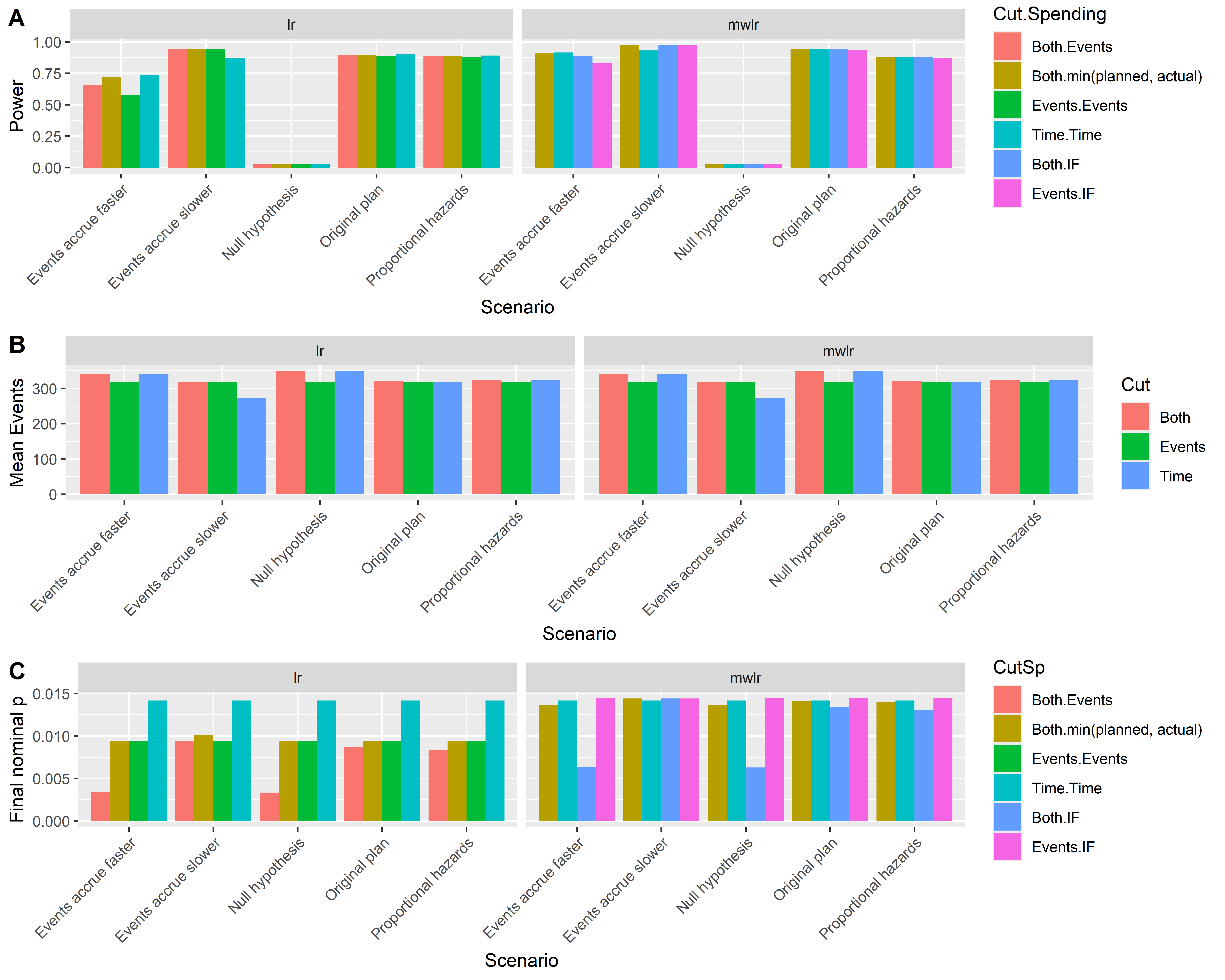
Summary
We have suggested the concept of spending time and provided 3 examples where the approach can be applied to simply adapt a design in a useful way. That is, if design assumptions are not met:
- execution is automatically adapted without protocol amendment,
- if there is a delayed treatment effect a trial can continue long enough and adequate \(\alpha\)-spending can be preserved to the final analysis where the full treatment effect can be realized and evaluated,
- if testing in multiple populations, spending can be automatically adapted so that \(\alpha\) is preserved until the final analysis and tests in all populations of interest can be maintained.
There are many potential solutions to issues that may arise related to error spending in group sequential trials. Michael A. Proschan, Lan, and Wittes (2006) discuss approaches such as using calendar time or adjusting future spending time on an adaptive basis at the time of analysis. We propose the concept of spending time as a more flexible alternative than information fraction for allocation of error spending between interim and final analyses in a group sequential trial. In particular, we have used spending time to ensure adequate Type I error spending is preserved for the final analysis in a trial, and timing of final analysis is not premature.
- For the case of a single endpoint where there may be a delayed treatment effect, we have proposed spending using the minimum of planned and observed information fraction at the time of an analysis. This is combined with potentially delaying the final analysis to achieve at least a minimum trial duration or follow-up duration for all study participants as well as achieving targeted events (statistical information).
- When testing multiple hypotheses on a single endpoint, we propose the minimum spending fraction based on all hypotheses being evaluated; this is in line with the suggestion of Follman, Proschan, and Geller (1994) for testing multiple experimental arms versus a common control in a group sequential trial. As an example, consider an oncology trial where both progression free survival (PFS) and overall survival (OS) are tested. Timing of interim analyses may be primarily determined by time and PFS event counts, while the final analysis is determined by time and OS event counts. Spending time can be used to determine interim and final \(\alpha\)-spending separately for PFS and OS in a way that adapts simply for all hypotheses tested. This includes the ability to use multiple testing procedures such as the graphical method of Maurer and Bretz (2013).
For the biomarker positive and overall population testing, adapting the overall sample size and spending based on enrolling the targeted biomarker positive sample size and spending according to events achieved in the biomarker subgroup for both population was effective at achieving targeted power and completing the trial in a timely fashion. The Fleming-Harrington-O’Brien spending approach mimicking Haybittle-Peto bounds was also effective at maintaining power and controlling Type I error. Depending on whether or not you wish to be conservative for early stopping (Haybittle-Peto) or more liberal with early stopping (O’Brien-Fleming-like bound), either approach can be used.
The scenarios considered are diverse, but not comprehensive. However, they illustrate several issues that should be considered at the time of design of a group sequential trial. Examples have been demonstrated with the design software of the gsDesign2 R package and the simulation R package simtrial.
Session info
sessioninfo::session_info(pkgs = "attached")#> ─ Session info ───────────────────────────────────────────────────────────────
#> setting value
#> version R version 4.5.1 (2025-06-13 ucrt)
#> os Windows 11 x64 (build 26100)
#> system x86_64, mingw32
#> ui RTerm
#> language (EN)
#> collate English_United States.utf8
#> ctype English_United States.utf8
#> tz America/New_York
#> date 2025-07-10
#> pandoc 3.7.0.2 @ C:/PROGRA~3/CHOCOL~1/bin/ (via rmarkdown)
#> quarto NA @ C:\\PROGRA~1\\RStudio\\RESOUR~1\\app\\bin\\quarto\\bin\\quarto.exe
#>
#> ─ Packages ───────────────────────────────────────────────────────────────────
#> package * version date (UTC) lib source
#> cowplot * 1.2.0 2025-07-07 [1] CRAN (R 4.5.1)
#> doFuture * 1.1.1 2025-06-06 [1] CRAN (R 4.5.0)
#> dplyr * 1.1.4 2023-11-17 [1] CRAN (R 4.5.0)
#> DT * 0.33 2024-04-04 [1] CRAN (R 4.5.0)
#> foreach * 1.5.2 2022-02-02 [1] CRAN (R 4.5.0)
#> future * 1.58.0 2025-06-05 [1] CRAN (R 4.5.0)
#> ggplot2 * 3.5.2 2025-04-09 [1] CRAN (R 4.5.0)
#> gsDesign * 3.6.9 2025-06-25 [1] CRAN (R 4.5.1)
#> gsDesign2 * 1.1.5 2025-06-27 [1] CRAN (R 4.5.1)
#> gt * 1.0.0 2025-04-05 [1] CRAN (R 4.5.0)
#> parallelly * 1.45.0 2025-06-02 [1] CRAN (R 4.5.0)
#> purrr * 1.0.4 2025-02-05 [1] CRAN (R 4.5.0)
#> simtrial * 1.0.0 2025-06-11 [1] CRAN (R 4.5.1)
#> tibble * 3.3.0 2025-06-08 [1] CRAN (R 4.5.0)
#> tictoc * 1.2.1 2024-03-18 [1] CRAN (R 4.5.0)
#>
#> [1] C:/Users/me/AppData/Local/R/win-library/4.5
#> [2] C:/Program Files/R/R-4.5.1/library
#> * ── Packages attached to the search path.
#>
#> ──────────────────────────────────────────────────────────────────────────────