---
title: "Multi-Endpoint Group Sequential Trial Simulation"
subtitle: "Illness-Death Model with OS, PFS, and ORR"
author: "Keaven M. Anderson"
date: "2026"
format:
html:
toc: true
code-fold: show
code-tools: true
---
```{r setup, message=FALSE, warning=FALSE}
library(gsDesign)
library(gMCPLite)
library(graphicalMCP)
library(survival)
library(data.table)
library(simtrial)
library(dplyr)
library(tidyr)
library(gt)
library(ggplot2)
library(parallel)

# Source illness-death model functions
source("../gMCPLite/inst/simulation/sim_illness_death.R")
source("../gMCPLite/inst/simulation/cut_illness_death.R")
```
## Design parameters
We design a two-arm (control vs. experimental) group sequential trial with
three endpoints: overall survival (OS), progression-free survival (PFS),
and objective response rate (ORR). The illness-death multi-state model
produces correlated endpoints from a single generative process.
**Key assumptions:**
- OS: control median 14 months, HR = 0.75
- PFS: HR = 0.75, piecewise control hazard (median 8 months for $t \in [0,8)$,
median 16 months for $t \geq 8$)
- ORR: control 15%, experimental 25%
- Enrollment: ramp-up over 6 months, 18 months total, 1:1 randomization
- Dropout: 1%/year (OS), 10%/year (PFS/ORR)
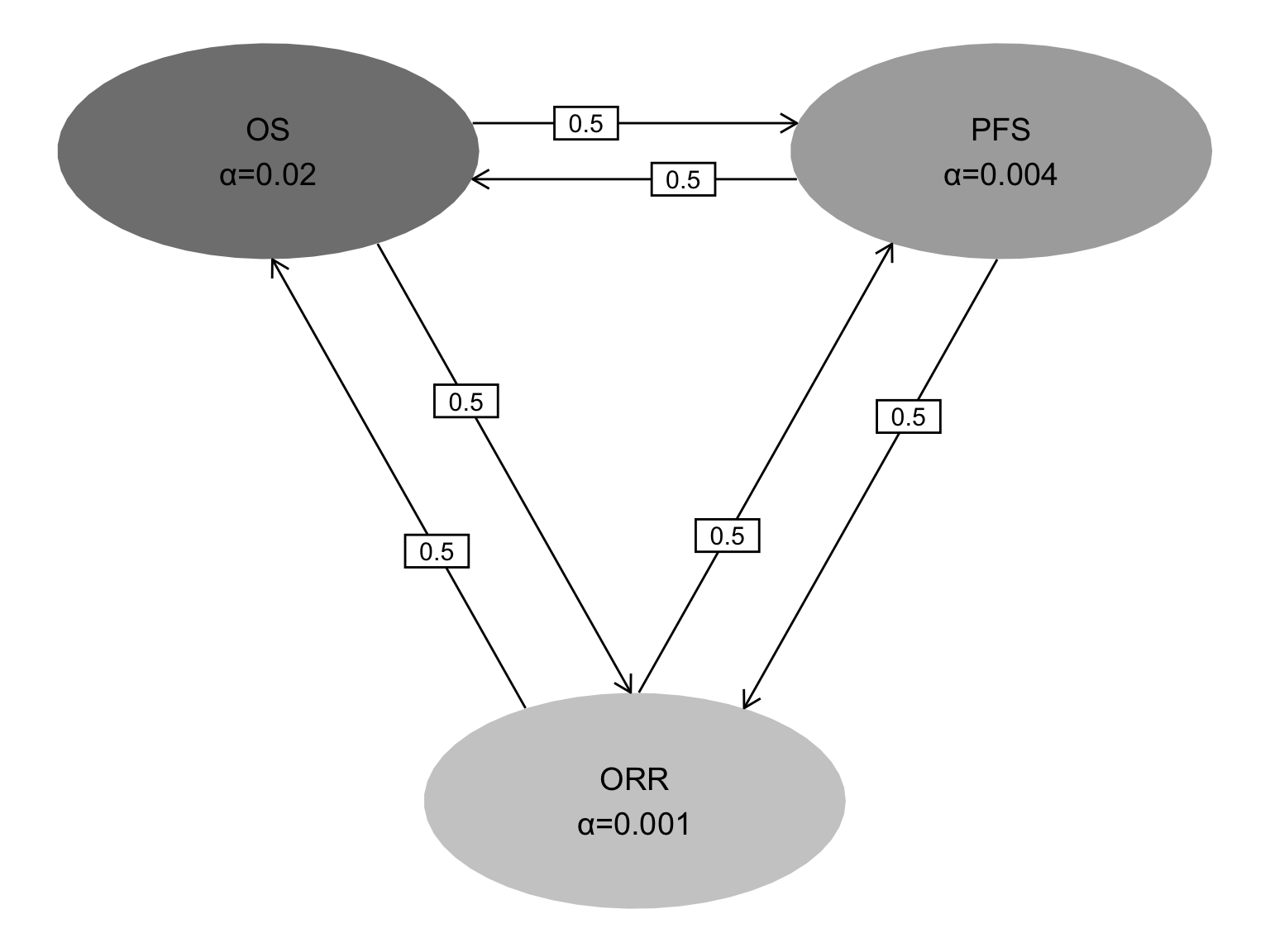
- Alpha allocation: OS = 0.02, PFS = 0.004, ORR = 0.001 (total = 0.025)
**Analysis timing:**
| Analysis | Month | Endpoints tested |
|----------|-------|-----------------|
| IA1 | 18 | PFS (efficacy + futility), OS (futility) |
| IA2 | 24 | ORR, PFS (efficacy), OS (futility) |
| IA3 | 30 | PFS (final), OS (efficacy) |
| FA | 42 | OS (efficacy) |
```{r parameters}
# Clinical assumptions
median_os_ctrl <- 14        # Control median OS (months)
hr_os <- 0.75               # OS hazard ratio
median_pfs_ctrl_1 <- 8      # Control median PFS, period 1 (months)
median_pfs_ctrl_2 <- 16     # Control median PFS, period 2 (months)
pfs_changepoint <- 8        # PFS hazard changepoint (months)
hr_pfs <- 0.75              # PFS hazard ratio
orr_ctrl <- 0.15            # Control ORR
orr_exp <- 0.25             # Experimental ORR
orr_changepoint <- 6        # Response rate changepoint (months)
orr_rate_mult <- 2.25       # Response rate multiplier for t < changepoint
orr_rate_late <- 0.1        # Late response rate as fraction of base rate

# Simulation effect sizes (weaker than design to reduce power)
sim_hr_os <- 0.80              # Simulation OS hazard ratio
sim_hr_pfs <- 0.80             # Simulation PFS hazard ratio

# Dropout rates (per month)
dropout_os <- -log(1 - 0.01) / 12     # 1%/year
dropout_pfs <- -log(1 - 0.10) / 12    # 10%/year

# Alpha allocation
alpha_os <- 0.02
alpha_pfs <- 0.004
alpha_orr <- 0.001
alpha_total <- alpha_os + alpha_pfs + alpha_orr  # 0.025

# Analysis times
analysis_times_os <- c(18, 24, 30, 42)   # OS: futility at 18, 24; efficacy at 30, 42
analysis_times_pfs <- c(18, 24, 30)       # PFS: fut+eff at 18, eff at 24, final at 30
analysis_time_orr <- 24                   # ORR at IA2 only

# Enrollment: ramp-up over 6 months, 18 months total
# Relative rates: 25%, 50%, 75%, 100% of steady state
enroll_duration <- c(2, 2, 2, 12)
enroll_rate_relative <- c(0.25, 0.50, 0.75, 1.00)
# Effective enrollment months = 0.25*2 + 0.5*2 + 0.75*2 + 1*12 = 15
```
## OS group sequential design (sample-size driving)
OS drives the sample size. We use `gsSurvCalendar()` with four analyses at
months 18, 24, 30, and 42. The 18- and 24-month interims have futility only
(no efficacy bound); efficacy testing begins at 30 months. No futility
bounds are applied at IA3 or FA via `testLower`. Futility spending uses
`sfExtremeValue2` to target an approximate HR of 0.9 at the futility bound.
```{r os-design}
# OS design using gsSurvCalendar()
# Futility at IA1 and IA2 only; no futility at IA3 or FA
os_design <- gsSurvCalendar(
  test.type = 4,
  alpha = alpha_os,
  beta = 0.1,
  sfu = sfLDOF,
  sfupar = NULL,
  sfl = sfExtremeValue2,
  sflpar = c(0.37, 0.9, 0.75, 0.95),
  testLower = c(TRUE, TRUE, FALSE, FALSE),
  calendarTime = c(18, 24, 30, 42),
  spending = "information",
  lambdaC = log(2) / median_os_ctrl,
  hr = hr_os,
  eta = dropout_os,
  gamma = enroll_rate_relative,
  R = enroll_duration,
  minfup = 24
) |> toInteger()

gsBoundSummary(os_design, timename = "Month", tdigits = 1,
               logdelta = TRUE, deltaname = "HR") |>
  gt() |>
  tab_header(title = paste0("OS Design (1-sided \u03b1 = ", alpha_os, ")"))
```
Extract sample size and enrollment rate from the OS design:
```{r os-extract}
# Total sample size (both arms)
n_total <- ceiling(sum(os_design$gamma * os_design$R))
cat("Total sample size:", n_total, "\n")
# Scaled enrollment rate (steady-state)
cat("Steady-state enrollment rate:",
    round(os_design$gamma[4], 1), "per month\n")
# Target OS events at each analysis
os_events <- os_design$n.I
cat("Target OS events:",
    paste(paste0("IA", 1:3, " = ", os_events[1:3]), collapse = ", "),
    ", FA =", os_events[4], "\n")
```
## PFS power
PFS has piecewise control hazard: median 8 months for $t < 8$, median 16
months for $t \geq 8$. We compute power with `gsSurvPower()` using the
enrollment from the OS design. Futility is applied only at IA1 (month 18)
via `testLower`; `sfExtremeValue2` targets ~HR = 0.9 at the futility bound.
```{r pfs-power}
# PFS power using gsSurvPower() with OS design enrollment
# Futility at IA1 only via testLower; sfExtremeValue2 targets ~HR=0.9
pfs_power <- gsSurvPower(
  k = 3,
  test.type = 4,
  alpha = alpha_pfs,
  sided = 1,
  sfu = sfLDOF,
  sfl = sfExtremeValue2,
  sflpar = c(0.6, 0.9, 0.15, 0.16),
  testLower = c(TRUE, FALSE, FALSE),
  lambdaC = log(2) / c(median_pfs_ctrl_1, median_pfs_ctrl_2),
  S = pfs_changepoint,
  hr = hr_pfs,
  eta = dropout_pfs,
  gamma = os_design$gamma,
  R = enroll_duration,
  ratio = 1,
  plannedCalendarTime = analysis_times_pfs
)

gsBoundSummary(pfs_power, timename = "Month", tdigits = 1,
               logdelta = TRUE, deltaname = "HR") |>
  gt() |>
  tab_header(title = paste0("PFS Design (1-sided \u03b1 = ", alpha_pfs, ")"))
```
```{r pfs-extract}
pfs_events <- ceiling(pfs_power$n.I)
cat("PFS events:",
    paste(paste0("IA", 1:2, " = ", pfs_events[1:2]), collapse = ", "),
    ", Final =", pfs_events[3], "\n")
# Cumulative power
cat("PFS cumulative power (1-sided \u03b1 =", alpha_pfs, "):",
    round(pfs_power$power, 3), "\n")
```
## ORR power
ORR is tested at IA2 only (month 24). We use `nBinomial()` for the
sample size calculation and power at the OS-driven sample size.
```{r orr-power}
# ORR sample size for 90% power (fixed design)
n_orr_fixed <- nBinomial(
  p1 = orr_ctrl,
  p2 = orr_exp,
  alpha = alpha_orr,
  beta = 0.1
)
cat("ORR fixed design sample size:", ceiling(n_orr_fixed), "\n")
# ORR power at the OS-driven sample size
n_orr <- n_total  # All enrolled by month 18, IA2 at month 24
beta_orr <- nBinomial(
  p1 = orr_ctrl,
  p2 = orr_exp,
  n = n_orr,
  alpha = alpha_orr
)
power_orr <- 1 - beta_orr
cat("ORR power at N =", n_orr,
    "(1-sided \u03b1 =", alpha_orr, "):",
    round(power_orr, 3), "\n")
cat("ORR effect size (risk difference):", orr_exp - orr_ctrl, "\n")
```
## Multiplicity graph
Symmetric graph with equal transition weights (0.5) between all three
hypotheses. Node labels show the allocated 1-sided $\alpha$ for each
hypothesis.
```{r graph, fig.width=8, fig.height=6}
# Create graph for multiplicity testing
g <- graph_create(
  hypotheses = c(OS = alpha_os / alpha_total,
                 PFS = alpha_pfs / alpha_total,
                 ORR = alpha_orr / alpha_total),
  transitions = rbind(
    c(0, 0.5, 0.5),   # From OS
    c(0.5, 0, 0.5),   # From PFS
    c(0.5, 0.5, 0)    # From ORR
  )
)

# Visualize with alpha values in nodes
hGraph(
  nHypotheses = 3,
  nameHypotheses = c("OS", "PFS", "ORR"),
  alphaHypotheses = c(alpha_os, alpha_pfs, alpha_orr),
  m = rbind(
    c(0, 0.5, 0.5),
    c(0.5, 0, 0.5),
    c(0.5, 0.5, 0)
  ),
  fill = c(1, 2, 3),
  halfWid = 1.0,
  halfHgt = 0.5,
  trhw = 0.15,
  trhh = 0.075,
  digits = 4,
  trdigits = 2,
  size = 5,
  boxtextsize = 4,
  trprop = 0.35
)
```
## Illness-death model
The simulation uses an illness-death multi-state model to generate
correlated OS, PFS, and ORR endpoints from a single generative process.
Patients start in State 0 (stable, no response) and transition between
states according to competing exponential hazards.
```{mermaid}
%%| fig-cap: "Illness-death model with response. Transitions are competing exponential hazards."
graph LR
  S0["<b>State 0</b><br/>Stable<br/>No Response"] -->|response| S1["<b>State 1</b><br/>Responded"]
  S0 -->|prog_0| S2["<b>State 2</b><br/>Progressed"]
  S0 -->|death_0| S3["<b>State 3</b><br/>Dead"]
  S1 -->|prog_1| S2
  S1 -->|death_1| S3
  S2 -->|death_2| S3
```
**Endpoint derivation:**
- **PFS**: time to first of progression (State 2) or death (State 3)
- **OS**: time to death (State 3)
- **ORR**: 1 if patient reaches State 1 (response) before progression or death
## Build illness-death transition rates
We calibrate the illness-death model using `build_transition_rates()` with
median PFS = 8 months (the first-period median), then modify the
transition rate table to implement piecewise PFS by halving the
progression rates after 8 months.
```{r transition-rates}
# Calibrate with first-period PFS median
transition_rate <- build_transition_rates(
  strata = "All",
  treatments = c("control", "experimental"),
  median_pfs = c(All = median_pfs_ctrl_1),
  median_os = c(All = median_os_ctrl),
  orr = list(All = c(control = orr_ctrl, experimental = orr_exp)),
  hr_pfs = c(All = hr_pfs),
  hr_os = c(All = hr_os)
)

# Display calibrated constant rates
transition_rate |>
  mutate(rate = round(rate, 4)) |>
  pivot_wider(names_from = treatment, values_from = rate) |>
  gt() |>
  tab_header(title = "Calibrated Transition Rates (Constant)")
```
### Implement piecewise rates
We modify two sets of transitions to be piecewise:
1. **Progression** (`prog_0`, `prog_1`): Half the rate after 8 months to
achieve piecewise PFS (median 8 months for $t < 8$, median 16 months
for $t \geq 8$).
2. **Response**: Multiply the rate by `r orr_rate_mult` for $t < 6$ months
so that the targeted ORR is largely achieved by 6 months, then drop to
`r 100 * orr_rate_late`% of the base rate for $t \geq 6$.
```{r piecewise-rates}
# Transitions to make piecewise
prog_transitions <- c("prog_0", "prog_1")

# Split constant-rate rows into piecewise rows
pw_rows <- list()
for (i in seq_len(nrow(transition_rate))) {
  row <- transition_rate[i, ]
  if (row$transition %in% prog_transitions) {
    # Period 1: original rate, duration = changepoint
    row1 <- row
    row1$duration <- pfs_changepoint
    pw_rows[[length(pw_rows) + 1]] <- row1
    # Period 2: half the rate, duration = Inf
    row2 <- row
    row2$rate <- row$rate / 2
    row2$duration <- Inf
    pw_rows[[length(pw_rows) + 1]] <- row2
  } else if (row$transition == "response") {
    # Period 1: high response rate for first 6 months
    row1 <- row
    row1$rate <- row$rate * orr_rate_mult
    row1$duration <- orr_changepoint
    pw_rows[[length(pw_rows) + 1]] <- row1
    # Period 2: much lower response rate after 6 months
    row2 <- row
    row2$rate <- row$rate * orr_rate_late
    row2$duration <- Inf
    pw_rows[[length(pw_rows) + 1]] <- row2
  } else {
    pw_rows[[length(pw_rows) + 1]] <- row
  }
}
transition_rate_pw <- do.call(rbind, pw_rows)

transition_rate_pw |>
  mutate(rate = round(rate, 4),
         duration = ifelse(is.infinite(duration), "Inf",
                           as.character(duration))) |>
  gt() |>
  tab_header(title = "Piecewise Transition Rates")
```
### Simulation transition rates
The simulation uses weaker treatment effects (OS HR = `r sim_hr_os`,
PFS HR = `r sim_hr_pfs`) than the design assumptions to evaluate
realistic operating characteristics.
```{r sim-transition-rates}
# Build transition rates with simulation-specific effect sizes
transition_rate_sim <- build_transition_rates(
  strata = "All",
  treatments = c("control", "experimental"),
  median_pfs = c(All = median_pfs_ctrl_1),
  median_os = c(All = median_os_ctrl),
  orr = list(All = c(control = orr_ctrl, experimental = orr_exp)),
  hr_pfs = c(All = sim_hr_pfs),
  hr_os = c(All = sim_hr_os)
)

# Apply same piecewise logic as design rates
pw_rows_sim <- list()
for (i in seq_len(nrow(transition_rate_sim))) {
  row <- transition_rate_sim[i, ]
  if (row$transition %in% prog_transitions) {
    row1 <- row; row1$duration <- pfs_changepoint
    pw_rows_sim[[length(pw_rows_sim) + 1]] <- row1
    row2 <- row; row2$rate <- row$rate / 2; row2$duration <- Inf
    pw_rows_sim[[length(pw_rows_sim) + 1]] <- row2
  } else if (row$transition == "response") {
    row1 <- row; row1$rate <- row$rate * orr_rate_mult; row1$duration <- orr_changepoint
    pw_rows_sim[[length(pw_rows_sim) + 1]] <- row1
    row2 <- row; row2$rate <- row$rate * orr_rate_late; row2$duration <- Inf
    pw_rows_sim[[length(pw_rows_sim) + 1]] <- row2
  } else {
    pw_rows_sim[[length(pw_rows_sim) + 1]] <- row
  }
}
transition_rate_pw_sim <- do.call(rbind, pw_rows_sim)
```
## Simulation
We simulate 1,000 trials using parallel processing with simulation
effect sizes (OS HR = `r sim_hr_os`, PFS HR = `r sim_hr_pfs`).
For each trial we compute test statistics and collect event counts
at each analysis for spending time computation:
| Month | Statistics |
|-------|-----------|
| 18 | $Z_\text{PFS}$ (logrank), $Z_\text{OS}$ (logrank) |
| 24 | $Z_\text{ORR}$ (risk difference), $Z_\text{PFS}$ (logrank), $Z_\text{OS}$ (logrank) |
| 30 | $Z_\text{PFS}$ (logrank), $Z_\text{OS}$ (logrank) |
| 42 | $Z_\text{OS}$ (logrank) |
### Test statistic functions
```{r test-functions}
# Logrank Z statistic via simtrial::wlr (positive = experimental better)
logrank_z <- function(data) {
  d <- data.frame(
    tte = data$AVAL,
    event = 1L - data$CNSR,
    stratum = data$STRATUM,
    treatment = data$TRT
  )
  if (sum(d$event) < 2) return(NA_real_)
  wlr(d, weight = fh(rho = 0, gamma = 0))$z
}

# Binomial Z statistic via gsDesign::testBinomial (positive = experimental better)
rd_z <- function(data) {
  n_ctrl <- sum(data$TRT == "control")
  n_exp <- sum(data$TRT == "experimental")
  if (n_exp == 0 || n_ctrl == 0) return(NA_real_)
  x_ctrl <- sum(data$AVAL[data$TRT == "control"])
  x_exp <- sum(data$AVAL[data$TRT == "experimental"])
  testBinomial(x1 = x_exp, x2 = x_ctrl, n1 = n_exp, n2 = n_ctrl)
}
```
### Run simulations
```{r simulate, cache=TRUE}
# Set up parallel backend
n_workers <- max(1, parallel::detectCores() - 2)

set.seed(20260404)
n_sim <- 1000

# Enrollment rate from OS design
enroll_rate_sim <- data.frame(
  rate = unname(os_design$gamma),
  duration = enroll_duration
)

# Single simulation function
run_one_sim <- function(sim_id) {
  tryCatch({
    sim_data <- sim_illness_death(
      n = n_total,
      stratum = data.frame(stratum = "All", p = 1),
      block = c("control", "control", "experimental", "experimental"),
      enroll_rate = enroll_rate_sim,
      transition_rate = transition_rate_pw_sim,
      dropout_rate = dropout_os
    )

    adtte_18 <- cut_illness_death(sim_data, cut_date = 18)
    adtte_24 <- cut_illness_death(sim_data, cut_date = 24)
    adtte_30 <- cut_illness_death(sim_data, cut_date = 30)
    adtte_42 <- cut_illness_death(sim_data, cut_date = 42)

    # Z statistics
    z_vals <- c(
      logrank_z(adtte_18[adtte_18$PARAMCD == "PFS", ]),
      logrank_z(adtte_18[adtte_18$PARAMCD == "OS", ]),
      rd_z(adtte_24[adtte_24$PARAMCD == "ORR", ]),
      logrank_z(adtte_24[adtte_24$PARAMCD == "PFS", ]),
      logrank_z(adtte_24[adtte_24$PARAMCD == "OS", ]),
      logrank_z(adtte_30[adtte_30$PARAMCD == "PFS", ]),
      logrank_z(adtte_30[adtte_30$PARAMCD == "OS", ]),
      logrank_z(adtte_42[adtte_42$PARAMCD == "OS", ])
    )

    # Event counts for spending time computation
    ev_vals <- c(
      sum(1L - adtte_18$CNSR[adtte_18$PARAMCD == "PFS"]),
      sum(1L - adtte_24$CNSR[adtte_24$PARAMCD == "PFS"]),
      sum(1L - adtte_30$CNSR[adtte_30$PARAMCD == "PFS"]),
      sum(1L - adtte_18$CNSR[adtte_18$PARAMCD == "OS"]),
      sum(1L - adtte_24$CNSR[adtte_24$PARAMCD == "OS"]),
      sum(1L - adtte_30$CNSR[adtte_30$PARAMCD == "OS"]),
      sum(1L - adtte_42$CNSR[adtte_42$PARAMCD == "OS"])
    )

    c(z_vals, ev_vals)
  }, error = function(e) rep(NA_real_, 15))
}

t_start <- proc.time()

z_list <- mclapply(
  seq_len(n_sim),
  run_one_sim,
  mc.cores = n_workers,
  mc.set.seed = TRUE
)

t_elapsed <- (proc.time() - t_start)[3]

sim_results <- do.call(rbind, z_list)
z_matrix <- sim_results[, 1:8]
colnames(z_matrix) <- c("Z_PFS_18", "Z_OS_18", "Z_ORR_24", "Z_PFS_24",
                         "Z_OS_24", "Z_PFS_30", "Z_OS_30", "Z_OS_42")
events_matrix <- sim_results[, 9:15]
colnames(events_matrix) <- c("PFS_18", "PFS_24", "PFS_30",
                              "OS_18", "OS_24", "OS_30", "OS_42")
n_failed <- sum(apply(sim_results, 1, function(r) all(is.na(r))))
cat("Simulations complete:", n_sim, "trials in",
    round(t_elapsed, 1), "seconds\n")
cat("Workers used:", n_workers, "\n")
if (n_failed > 0) cat("Failed simulations:", n_failed, "\n")
cat("Missing values (Z):",
    sum(is.na(z_matrix)), "of", prod(dim(z_matrix)), "\n")
```
## Results
### Sequential testing
For each simulated trial, we compute sequential p-values at each analysis
using `sequentialPValue()` with spending time =
$\min(\text{planned events}, \text{actual events}) / \text{planned final events}$
at interim analyses and spending time = 1 at final analyses. For ORR
(fixed-sample test at IA2), the nominal one-sided p-value is used. The
sequential p-values are tested using `graph_test_shortcut()` at each
analysis, with the multiplicity graph controlling the familywise error
rate at $\alpha = `r alpha_total`$.
```{r sequential-testing}
# Planned events from designs
planned_os_ev <- os_design$n.I    # 4 values for months 18, 24, 30, 42
planned_pfs_ev <- pfs_power$n.I   # 3 values for months 18, 24, 30

# Track first rejection analysis for each hypothesis
# Analyses: 1=IA1(18mo), 2=IA2(24mo), 3=IA3(30mo), 4=FA(42mo)
first_rej <- matrix(NA_integer_, nrow = n_sim, ncol = 3,
                    dimnames = list(NULL, c("OS", "PFS", "ORR")))

for (i in seq_len(n_sim)) {
  if (any(is.na(z_matrix[i, ]))) next

  # Z values by endpoint
  z_pfs <- as.numeric(z_matrix[i, c("Z_PFS_18", "Z_PFS_24", "Z_PFS_30")])
  z_os <- as.numeric(z_matrix[i, c("Z_OS_18", "Z_OS_24", "Z_OS_30", "Z_OS_42")])
  z_orr <- as.numeric(z_matrix[i, "Z_ORR_24"])

  # Event counts by endpoint
  ev_pfs <- as.numeric(events_matrix[i, c("PFS_18", "PFS_24", "PFS_30")])
  ev_os <- as.numeric(events_matrix[i, c("OS_18", "OS_24", "OS_30", "OS_42")])

  # ORR nominal p-value (one-sided, positive Z = experimental better)
  p_orr_nom <- pnorm(-z_orr)

  rejected <- c(OS = FALSE, PFS = FALSE, ORR = FALSE)
  p_pfs_cur <- 1
  p_orr_cur <- 1

  for (k in 1:4) {
    # OS sequential p-value (all 4 analyses)
    st_os <- pmin(planned_os_ev[1:k], ev_os[1:k]) / planned_os_ev[4]
    if (k == 4) st_os[4] <- 1
    p_os_cur <- tryCatch(
      sequentialPValue(os_design, n.I = ev_os[1:k],
                       Z = z_os[1:k], usTime = st_os),
      error = function(e) 1
    )

    # PFS sequential p-value (3 analyses: months 18, 24, 30)
    if (k <= 3) {
      st_pfs <- pmin(planned_pfs_ev[1:k], ev_pfs[1:k]) / planned_pfs_ev[3]
      if (k == 3) st_pfs[3] <- 1
      p_pfs_cur <- tryCatch(
        sequentialPValue(pfs_power, n.I = ev_pfs[1:k],
                         Z = z_pfs[1:k], usTime = st_pfs),
        error = function(e) 1
      )
    }
    # else: carry forward p_pfs_cur from k=3

    # ORR: nominal p-value from IA2 onwards
    if (k >= 2) p_orr_cur <- p_orr_nom

    # Graphical multiplicity testing
    result <- graph_test_shortcut(g,
      p = c(p_os_cur, p_pfs_cur, p_orr_cur),
      alpha = alpha_total
    )

    # Record first rejection
    rej_now <- result$outputs$rejected
    newly <- rej_now & !rejected
    if (any(newly)) {
      first_rej[i, which(newly)] <- k
    }
    rejected <- rejected | rej_now

    if (all(rejected)) break
  }
}

cat("Sequential testing complete for", n_sim, "trials\n")
```
### Cumulative rejection probability
```{r rejection-summary}
# Analysis labels
analysis_labs <- c("IA1 (18 mo)", "IA2 (24 mo)", "IA3 (30 mo)", "FA (42 mo)")

# Build cumulative rejection table
rej_tab <- data.frame(Hypothesis = c("OS", "PFS", "ORR"))
for (k in 1:4) {
  rej_tab[[analysis_labs[k]]] <- sapply(1:3, function(h) {
    sum(first_rej[, h] <= k, na.rm = TRUE)
  })
}

rej_tab |>
  gt() |>
  tab_header(
    title = paste("Cumulative Rejections by Analysis (", n_sim, "simulations)"),
    subtitle = paste0("Simulation HR: OS = ", sim_hr_os, ", PFS = ", sim_hr_pfs,
                      ". ORR: ctrl = ", orr_ctrl, ", exp = ", orr_exp)
  )
```
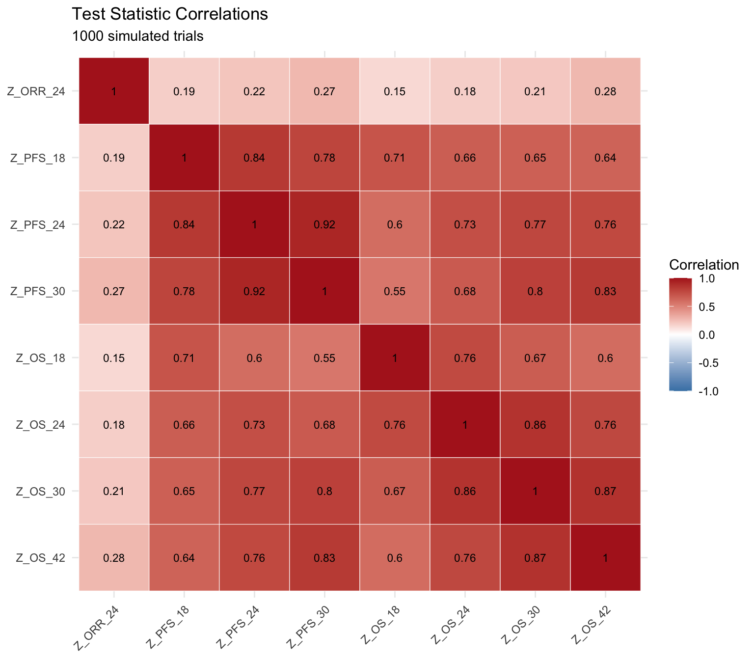
### Estimated correlation matrix
The correlation between test statistics across the 8 analysis--endpoint
combinations informs the joint distribution needed for multiplicity
adjustment.
```{r correlation}
# Reorder columns for display
col_order <- c("Z_ORR_24", "Z_PFS_18", "Z_PFS_24", "Z_PFS_30",
               "Z_OS_18", "Z_OS_24", "Z_OS_30", "Z_OS_42")
z_ordered <- z_matrix[, col_order]
cor_matrix <- cor(z_ordered, use = "pairwise.complete.obs")

cor_matrix |>
  round(3) |>
  as.data.frame() |>
  tibble::rownames_to_column("Statistic") |>
  gt() |>
  tab_header(
    title = "Estimated Correlation Matrix",
    subtitle = paste(n_sim, "simulated trials")
  ) |>
  fmt_number(columns = -Statistic, decimals = 3)
```
### Correlation heatmap
```{r heatmap, fig.width=8, fig.height=7}
# Reshape for plotting
cor_long <- cor_matrix |>
  as.data.frame() |>
  tibble::rownames_to_column("Var1") |>
  pivot_longer(-Var1, names_to = "Var2", values_to = "Correlation")

# Order factor levels
cor_long$Var1 <- factor(cor_long$Var1, levels = rev(col_order))
cor_long$Var2 <- factor(cor_long$Var2, levels = col_order)

ggplot(cor_long, aes(x = Var2, y = Var1, fill = Correlation)) +
  geom_tile(color = "white") +
  geom_text(aes(label = round(Correlation, 2)), size = 3) +
  scale_fill_gradient2(low = "steelblue", mid = "white", high = "firebrick",
                       midpoint = 0, limits = c(-1, 1)) +
  labs(title = "Test Statistic Correlations",
       subtitle = paste(n_sim, "simulated trials"),
       x = NULL, y = NULL) +
  theme_minimal() +
  theme(axis.text.x = element_text(angle = 45, hjust = 1))
```
### Event counts at each analysis
```{r events}
# Run one trial to show typical event counts
set.seed(1)
sim_example <- sim_illness_death(
  n = n_total,
  stratum = data.frame(stratum = "All", p = 1),
  block = c("control", "control", "experimental", "experimental"),
  enroll_rate = enroll_rate_sim,
  transition_rate = transition_rate_pw_sim,
  dropout_rate = dropout_os
)

# Planned events from designs
planned_os <- os_design$n.I          # 4 values: months 18, 24, 30, 42
planned_pfs <- pfs_power$n.I         # 3 values: months 18, 24, 30
planned_orr <- round(n_total * (orr_ctrl + orr_exp) / 2)  # Expected under H1

event_counts <- data.frame(
  Analysis = c("IA1 (18 mo)", "IA2 (24 mo)", "IA3 (30 mo)", "FA (42 mo)"),
  cut_date = c(18, 24, 30, 42)
) |>
  rowwise() |>
  mutate(
    adtte = list(cut_illness_death(sim_example, cut_date)),
    N_enrolled = sum(adtte$PARAMCD == "OS"),
    OS_planned = planned_os[which(c(18, 24, 30, 42) == cut_date)],
    OS_actual = sum(adtte$CNSR[adtte$PARAMCD == "OS"] == 0),
    PFS_planned = ifelse(cut_date <= 30,
                         ceiling(planned_pfs[which(c(18, 24, 30) == cut_date)]),
                         NA_integer_),
    PFS_actual = sum(adtte$CNSR[adtte$PARAMCD == "PFS"] == 0),
    ORR_expected = ifelse(cut_date == 24, planned_orr, NA_integer_),
    ORR_actual = sum(adtte$AVAL[adtte$PARAMCD == "ORR"])
  ) |>
  select(Analysis, N_enrolled,
         OS_planned, OS_actual,
         PFS_planned, PFS_actual,
         ORR_expected, ORR_actual)

event_counts |>
  ungroup() |>
  gt() |>
  tab_header(title = "Event Counts: Planned vs. Actual (Example Trial)") |>
  cols_label(
    OS_planned = "Planned", OS_actual = "Actual",
    PFS_planned = "Planned", PFS_actual = "Actual",
    ORR_expected = "Expected", ORR_actual = "Actual"
  ) |>
  tab_spanner(label = "OS Events", columns = c(OS_planned, OS_actual)) |>
  tab_spanner(label = "PFS Events", columns = c(PFS_planned, PFS_actual)) |>
  tab_spanner(label = "ORR Responses", columns = c(ORR_expected, ORR_actual)) |>
  sub_missing(missing_text = "--")
```
## Notes
1. **Piecewise PFS approximation**: The piecewise control PFS is
implemented by halving the progression rates (`prog_0`, `prog_1`) after
8 months. This is an approximation; the actual marginal PFS median in
the second period depends on the full competing risks structure.
2. **Single dropout rate**: The illness-death model uses a single dropout
rate applied to all endpoints. We use the OS dropout rate (1%/year) for
the simulation. The higher PFS dropout rate (10%/year) is used only in
the gsDesign power calculations. In practice, PFS-specific censoring
(e.g., missed tumor assessments) could be layered on top.
3. **Correlation interpretation**: High correlations between the same
endpoint at different analyses (e.g., $Z_\text{PFS}$ at months 16 and 24)
reflect the incremental information structure. Cross-endpoint
correlations (e.g., PFS and OS) reflect the biological coupling through
the illness-death model.
4. **Simulation size**: With `r n_sim` simulations, the standard error of each
correlation estimate is approximately $1/\sqrt{`r n_sim`}
= `r round(1/sqrt(n_sim), 3)`$.
5. **Enrollment**: The simulation uses Poisson process enrollment via
`rpwexp_enroll()`. Enrollment rates are taken directly from the OS
design so that the expected total matches the designed sample size.
Actual enrollment duration varies slightly across simulations.
## Session information
```{r session-info}
sessionInfo()
```