lambdaC <- log(2) / 20
hr <- .5
hr0 <- 1
S <- NULL
T <- 30
R <- 20
minfup <- 10
gamma <- 8
alpha <- .025
sided <- 1
beta <- .1
etaC <- 0
etaE <- 0
ratio <- 13 Examples for fixed design sample size and power
We present examples for the advanced time-to-event sample size routine nSurv(), corresponding to four types of calculations. All assume an input hazard ratio, dropout rates, and Type I error rate. The first three assume an input Type II error rate, while the fourth computes power. The types of calculations are:
- Based on a fixed enrollment duration and follow-up period, derive the enrollment rates required to obtain adequate power (Lachin and Foulkes 1986).
- Based on fixed enrollment rates and a fixed minimum follow-up period, derive accrual duration required to obtain adequate power (Kim and Tsiatis 1990).
- Based on fixed enrollment rates and accrual duration, derive study duration required to obtain adequate power (Kim and Tsiatis 1990).
- Based on fixed accrual duration, accrual rates and follow-up, derive study power.
3.1 Setup
The first four examples reuse a common set of assumptions.
3.2 Derive accrual rates
We begin by specifying values for all four of 1) control event rates (lambdaC), 2) accrual duration (R), 3) minimum follow-up (minfup), and trial duration (T). Relative accrual rates are specified in gamma for the time periods specified in R; these are modified on output to give absolute accrual rates required to achieve the desired power.
x <- nSurv(
  lambdaC = lambdaC, hr = hr, hr0 = hr0, eta = etaC, etaE = etaE,
  gamma = gamma, R = R, S = S, T = T, minfup = minfup, ratio = ratio,
  alpha = alpha, beta = beta
)
print(x)
nSurv fixed-design summary (method=LachinFoulkes; target=Accrual rate)
HR=0.500 vs HR0=1.000 | alpha=0.025 (sided=1) | power=90.0%
N=227.6 subjects | D=88.7 events | T=30.0 study duration | accrual=20.0 Accrual duration | minfup=10.0 minimum follow-up | ratio=1 randomization ratio (experimental/control)
Key inputs (names preserved):
desc item value input
Accrual rate(s) gamma 11.381 8
Accrual rate duration(s) R 20 20
Control hazard rate(s) lambdaC 0.035 0.035
Control dropout rate(s) eta 0 0
Experimental dropout rate(s) etaE 0 0
Event and dropout rate duration(s) S NULL S3.3 Derive duration for accrual and study
Now we set the input study duration (T) to NULL so that it can be adjusted to achieve desired power; enrollment duration is altered to total study duration minus the input minimum follow-up.
x <- nSurv(
  lambdaC = lambdaC, hr = hr, hr0 = hr0, eta = etaC, etaE = etaE,
  gamma = gamma, R = R, S = S, T = NULL, minfup = minfup, ratio = ratio,
  alpha = alpha, beta = beta
)
x
nSurv fixed-design summary (method=LachinFoulkes; target=Accrual duration)
HR=0.500 vs HR0=1.000 | alpha=0.025 (sided=1) | power=90.0%
N=206.7 subjects | D=88.4 events | T=35.8 study duration | accrual=25.8 Accrual duration | minfup=10.0 minimum follow-up | ratio=1 randomization ratio (experimental/control)
Key inputs (names preserved):
desc item value input
Accrual rate(s) gamma 8 8
Accrual rate duration(s) R 25.836 20
Control hazard rate(s) lambdaC 0.035 0.035
Control dropout rate(s) eta 0 0
Experimental dropout rate(s) etaE 0 0
Event and dropout rate duration(s) S NULL S3.4 Derive follow-up duration
Next we set the input follow-up (minfup) to NULL so that it can be derived to achieve the desired power. Note that this strategy will often fail if accrual is too little or too much in the specified time period. Thus, it is often easier to allow study and accrual duration to vary as in the previous nsurv_example_setup.
x <- nSurv(
  lambdaC = lambdaC, hr = hr, hr0 = hr0, eta = etaC, etaE = etaE,
  gamma = gamma, R = R, S = S, T = T, minfup = NULL, ratio = ratio,
  alpha = alpha, beta = beta
)
x
nSurv fixed-design summary (method=LachinFoulkes; target=Follow-up duration)
HR=0.500 vs HR0=1.000 | alpha=0.025 (sided=1) | power=90.0%
N=160.0 subjects | D=87.6 events | T=42.4 study duration | accrual=20.0 Accrual duration | minfup=22.4 minimum follow-up | ratio=1 randomization ratio (experimental/control)
Key inputs (names preserved):
desc item value input
Accrual rate(s) gamma 8 8
Accrual rate duration(s) R 20 20
Control hazard rate(s) lambdaC 0.035 0.035
Control dropout rate(s) eta 0 0
Experimental dropout rate(s) etaE 0 0
Event and dropout rate duration(s) S NULL S3.5 Derive power
Finally, we compute the power for a design by setting the input beta to NULL. In this case, all of 1) R (accrual rate periods), 2) gamma (accrual rates in specified periods), 3) T (trial duration), and 4) minfup (minimum follow-up after accrual) must be specified.
nSurv(
  lambdaC = lambdaC, hr = hr, hr0 = hr0, eta = etaC, etaE = etaE,
  gamma = gamma, R = R, S = S, T = T, minfup = minfup, ratio = ratio,
  alpha = alpha, beta = NULL
)
nSurv fixed-design summary (method=LachinFoulkes; target=Power)
HR=0.500 vs HR0=1.000 | alpha=0.025 (sided=1) | power=78.0%
N=160.0 subjects | D=62.3 events | T=30.0 study duration | accrual=20.0 Accrual duration | minfup=10.0 minimum follow-up | ratio=1 randomization ratio (experimental/control)
Key inputs (names preserved):
desc item value input
Accrual rate(s) gamma 8 8
Accrual rate duration(s) R 20 20
Control hazard rate(s) lambdaC 0.035 0.035
Control dropout rate(s) eta 0 0
Experimental dropout rate(s) etaE 0 0
Event and dropout rate duration(s) S NULL S
3.6 Examples with alternative method argument
We compare the four method options using a single-stratum, exponential setup similar to Schoenfeld (1981) (1981) and Freedman (1982) (1982), and the Bernstein and Lagakos rates above. This illustrates how required sample size and events differ when the variance formulation changes. Generally, we recommend the Lachin and Foulkes method due to accuracy. Often there is very little difference between the Schoenfeld and Lachin and Foulkes methods. The Bernstein and Lagakos method can give a sample size that is too small, but we have included it for historical purposes. The Freedman method can be a bit more conservative with a larger sample size. It is worth considering simulations if you wish to confirm power calculations.
lambdaC <- log(2) / 6
method_list <- c("LachinFoulkes", "Schoenfeld",
                 "Freedman", "BernsteinLagakos")
# Using nSurv() (current approach)
method_out <- lapply(
  method_list,
  function(m) {
    nSurv(
      alpha = .025, beta = .1, lambdaC = lambdaC, hr = .6,
      hr0 = 1, ratio = 1, R = 24, T = 36, minfup = 12,
      method = m
    )
  }
)
res <- do.call(
  rbind,
  Map(
    function(nm, obj) {
      data.frame(
        method = nm,
        n = obj$n,
        events = obj$d
      )
    },
    method_list, method_out
  )
)
res
method n events
LachinFoulkes LachinFoulkes 187.4523 159.6519
Schoenfeld Schoenfeld 189.1156 161.0686
Freedman Freedman 197.3935 168.1188
BernsteinLagakos BernsteinLagakos 181.5053 154.58693.7 Comparison with rpact (example)
The rpact package provides similar calculations via getSampleSizeSurvival(). Below we align parameters with the simple exponential example (control hazard log(2)/6, HR = 0.6, 24 months accrual and 12 months follow-up). The results to degree of accuracy shown are the same as with nSurv() above.
# Install rpact if not available
if (!require("rpact", quietly = TRUE)) {
  install.packages("rpact", repos = "https://cran.rstudio.com/")
  library(rpact)
}

# Control hazard = log(2)/6; experimental = HR * control
lambda2 <- log(2) / 6          # control

# One-look design matching the nSurv setup (1-sided alpha=0.025, beta=0.1)
design1 <- getDesignGroupSequential(
  kMax = 1, alpha = 0.025, beta = 0.1, sided = 1
)

# Schoenfeld (default), ratio = 1
rp_schoen <- getSampleSizeSurvival(
  design = design1,
  lambda2 = lambda2, hazardRatio = 0.6,
  accrualTime = 24, followUpTime = 12,
  dropoutRate1 = 0, dropoutRate2 = 0
)

# Schoenfeld, ratio = 2
rp_schoen_r2 <- getSampleSizeSurvival(
  design = design1,
  lambda2 = lambda2, hazardRatio = 0.6,
  accrualTime = 24, followUpTime = 12,
  dropoutRate1 = 0, dropoutRate2 = 0,
  allocationRatioPlanned = 2
)

# Schoenfeld, ratio = 0.5
rp_schoen_r05 <- getSampleSizeSurvival(
  design = design1,
  lambda2 = lambda2, hazardRatio = 0.6,
  accrualTime = 24, followUpTime = 12,
  dropoutRate1 = 0, dropoutRate2 = 0,
  allocationRatioPlanned = 0.5
)

# Freedman, ratio = 1
rp_freed <- getSampleSizeSurvival(
  design = design1,
  lambda2 = lambda2, hazardRatio = 0.6,
  accrualTime = 24, followUpTime = 12,
  dropoutRate1 = 0, dropoutRate2 = 0,
  typeOfComputation = "Freedman"
)

# Freedman, ratio = 2
rp_freed_r2 <- getSampleSizeSurvival(
  design = design1,
  lambda2 = lambda2, hazardRatio = 0.6,
  accrualTime = 24, followUpTime = 12,
  dropoutRate1 = 0, dropoutRate2 = 0,
  allocationRatioPlanned = 2,
  typeOfComputation = "Freedman"
)

# Freedman, ratio = 0.5
rp_freed_r05 <- getSampleSizeSurvival(
  design = design1,
  lambda2 = lambda2, hazardRatio = 0.6,
  accrualTime = 24, followUpTime = 12,
  dropoutRate1 = 0, dropoutRate2 = 0,
  allocationRatioPlanned = 0.5,
  typeOfComputation = "Freedman"
)

rp_tab <- rbind(
  data.frame(
    source = "nSurv", method = "Schoenfeld", ratio = 0.5,
    n = nSurv(
      lambdaC = lambda2, hr = 0.6, eta = 0,
      R = 24, T = 36, minfup = 12, ratio = 0.5,
      method = "Schoenfeld"
    )$n,
    events = nSurv(
      lambdaC = lambda2, hr = 0.6, eta = 0,
      R = 24, T = 36, minfup = 12, ratio = 0.5,
      method = "Schoenfeld"
    )$d
  ),
  data.frame(
    source = "nSurv", method = "Schoenfeld", ratio = 1,
    n = nSurv(
      lambdaC = lambda2, hr = 0.6, eta = 0,
      R = 24, T = 36, minfup = 12, ratio = 1,
      method = "Schoenfeld"
    )$n,
    events = nSurv(
      lambdaC = lambda2, hr = 0.6, eta = 0,
      R = 24, T = 36, minfup = 12, ratio = 1,
      method = "Schoenfeld"
    )$d
  ),
  data.frame(
    source = "nSurv", method = "Schoenfeld", ratio = 2,
    n = nSurv(
      lambdaC = lambda2, hr = 0.6, eta = 0,
      R = 24, T = 36, minfup = 12, ratio = 2,
      method = "Schoenfeld"
    )$n,
    events = nSurv(
      lambdaC = lambda2, hr = 0.6, eta = 0,
      R = 24, T = 36, minfup = 12, ratio = 2,
      method = "Schoenfeld"
    )$d
  ),
  data.frame(
    source = "nSurv", method = "Freedman", ratio = 0.5,
    n = nSurv(
      lambdaC = lambda2, hr = 0.6, eta = 0,
      R = 24, T = 36, minfup = 12, ratio = 0.5,
      method = "Freedman"
    )$n,
    events = nSurv(
      lambdaC = lambda2, hr = 0.6, eta = 0,
      R = 24, T = 36, minfup = 12, ratio = 0.5,
      method = "Freedman"
    )$d
  ),
  data.frame(
    source = "nSurv", method = "Freedman", ratio = 1,
    n = nSurv(
      lambdaC = lambda2, hr = 0.6, eta = 0,
      R = 24, T = 36, minfup = 12, ratio = 1,
      method = "Freedman"
    )$n,
    events = nSurv(
      lambdaC = lambda2, hr = 0.6, eta = 0,
      R = 24, T = 36, minfup = 12, ratio = 1,
      method = "Freedman"
    )$d
  ),
  data.frame(
    source = "nSurv", method = "Freedman", ratio = 2,
    n = nSurv(
      lambdaC = lambda2, hr = 0.6, eta = 0,
      R = 24, T = 36, minfup = 12, ratio = 2,
      method = "Freedman"
    )$n,
    events = nSurv(
      lambdaC = lambda2, hr = 0.6, eta = 0,
      R = 24, T = 36, minfup = 12, ratio = 2,
      method = "Freedman"
    )$d
  ),
  data.frame(
    source = "rpact", method = "Schoenfeld", ratio = 1,
    n = rp_schoen$maxNumberOfSubjects[1],
    events = rp_schoen$maxNumberOfEvents[1]
  ),
  data.frame(
    source = "rpact", method = "Schoenfeld", ratio = 2,
    n = rp_schoen_r2$maxNumberOfSubjects[1],
    events = rp_schoen_r2$maxNumberOfEvents[1]
  ),
  data.frame(
    source = "rpact", method = "Schoenfeld", ratio = 0.5,
    n = rp_schoen_r05$maxNumberOfSubjects[1],
    events = rp_schoen_r05$maxNumberOfEvents[1]
  ),
  data.frame(
    source = "rpact", method = "Freedman", ratio = 1,
    n = rp_freed$maxNumberOfSubjects[1],
    events = rp_freed$maxNumberOfEvents[1]
  ),
  data.frame(
    source = "rpact", method = "Freedman", ratio = 2,
    n = rp_freed_r2$maxNumberOfSubjects[1],
    events = rp_freed_r2$maxNumberOfEvents[1]
  ),
  data.frame(
    source = "rpact", method = "Freedman", ratio = 0.5,
    n = rp_freed_r05$maxNumberOfSubjects[1],
    events = rp_freed_r05$maxNumberOfEvents[1]
  )
)

rp_tab <- rp_tab[order(rp_tab$ratio, rp_tab$method, rp_tab$source), ]

rp_tab
source method ratio n events
4 nSurv Freedman 0.5 254.2745 221.9693
12 rpact Freedman 0.5 254.2745 221.9693
1 nSurv Schoenfeld 0.5 207.5742 181.2022
9 rpact Schoenfeld 0.5 207.5742 181.2022
5 nSurv Freedman 1.0 197.3935 168.1188
10 rpact Freedman 1.0 197.3935 168.1188
2 nSurv Schoenfeld 1.0 189.1156 161.0686
7 rpact Schoenfeld 1.0 189.1156 161.0686
6 nSurv Freedman 2.0 191.3751 158.9248
11 rpact Freedman 2.0 191.3751 158.9248
3 nSurv Schoenfeld 2.0 218.2013 181.2022
8 rpact Schoenfeld 2.0 218.2013 181.20223.8 Comparing methods across a range of hazard ratios
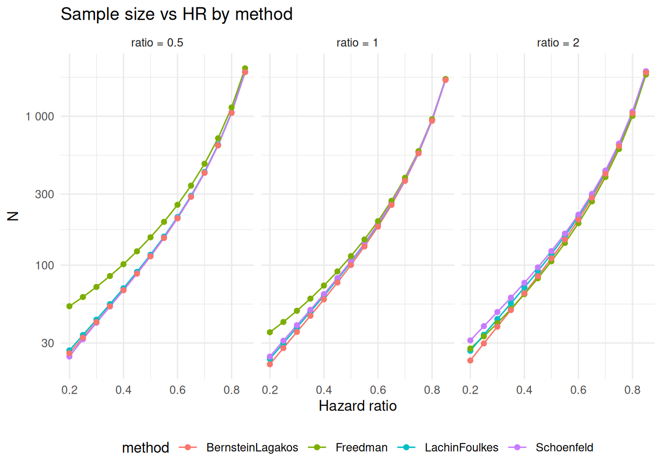
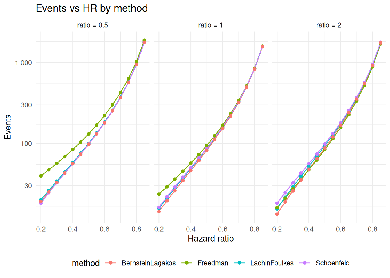
We continue the examples above by comparing sample size and targeted events by method for alternate hazard ratios from 0.2 to 0.85. We do this for ratio=.5, 1, 2. Summary plots comparing results are presented. The primary plot of likely interest with ratio = 1, equal randomization between treatment groups. We see that for very small hazard ratios that sample sizes can differ in a meaningful way with a large sample size and event count recommended by the Freedman method. For such cases, simulation studies may be worthwhile to further evaluate power.
if (plot_has_ggplot) {
  label_fun <- if (plot_has_scales) {
    scales::label_number()
  } else {
    ggplot2::waiver()
  }
  p_n <- ggplot2::ggplot(out, ggplot2::aes(x = hr, y = n, color = method)) +
    ggplot2::geom_line() +
    ggplot2::geom_point() +
    ggplot2::scale_y_log10(labels = label_fun) +
    ggplot2::facet_wrap(~ ratio, labeller = ggplot2::labeller(ratio = ratio_labels)) +
    ggplot2::labs(title = "Sample size vs HR by method", subtitle = "ratio = experimental:control randomization ratio", y = "N", x = "Hazard ratio") +
    ggplot2::theme_minimal() +
    ggplot2::theme(legend.position = "bottom", plot.title = ggplot2::element_text(hjust = 0.5), plot.subtitle = ggplot2::element_text(hjust = 0.5))
  print(p_n)
} else {
  op <- par(mfrow = c(1, length(ratio_grid)))
  on.exit(par(op), add = TRUE)
  for (r in ratio_grid) {
    subset_r <- out[out$ratio == r, ]
    y_n <- sapply(methods, function(m) subset_r$n[subset_r$method == m], simplify = "array")
    matplot(
      x = hr_grid,
      y = y_n,
      type = "l", lty = 1, main = paste("N vs HR (ratio=", r, ")"),
      xlab = "HR", ylab = "N", log = "y", yaxt = "n"
    )
    axis(2, at = 10^pretty(log10(range(y_n))), labels = 10^pretty(log10(range(y_n))))
    matpoints(x = hr_grid, y = y_n, pch = 16)
    legend("topright", legend = methods, col = 1:length(methods), lty = 1, pch = 16, bty = "n")
  }
}
if (plot_has_ggplot) {
  label_fun <- if (plot_has_scales) {
    scales::label_number()
  } else {
    ggplot2::waiver()
  }
  p_events <- ggplot2::ggplot(out, ggplot2::aes(x = hr, y = events, color = method)) +
    ggplot2::geom_line() +
    ggplot2::geom_point() +
    ggplot2::scale_y_log10(labels = label_fun) +
    ggplot2::facet_wrap(~ ratio, labeller = ggplot2::labeller(ratio = ratio_labels)) +
    ggplot2::labs(title = "Events vs HR by method", subtitle = "ratio = experimental:control randomization ratio", y = "Events", x = "Hazard ratio") +
    ggplot2::theme_minimal() +
    ggplot2::theme(legend.position = "bottom", plot.title = ggplot2::element_text(hjust = 0.5), plot.subtitle = ggplot2::element_text(hjust = 0.5))
  print(p_events)
} else {
  op <- par(mfrow = c(1, length(ratio_grid)))
  on.exit(par(op), add = TRUE)
  for (r in ratio_grid) {
    subset_r <- out[out$ratio == r, ]
    y_e <- sapply(methods, function(m) subset_r$events[subset_r$method == m], simplify = "array")
    matplot(
      x = hr_grid,
      y = y_e,
      type = "l", lty = 1, main = paste("Events vs HR (ratio=", r, ")"),
      xlab = "HR", ylab = "Events", log = "y", yaxt = "n"
    )
    axis(2, at = 10^pretty(log10(range(y_e))), labels = 10^pretty(log10(range(y_e))))
    matpoints(x = hr_grid, y = y_e, pch = 16)
    legend("topright", legend = methods, col = 1:length(methods), lty = 1, pch = 16, bty = "n")
  }
}
3.9 Non-inferiority and super-superiority
The method options extend to non-inferiority (NI) and very strong superiority settings. Below, NI uses a margin of HR = 1.25 with an expected HR = 1.05 (treatment slightly worse than control), while the super-superiority scenario uses HR = 0.5 with HR = 0.9 under the null hypothesis with unequal randomization 2:1. Note that only superiority testing is supported for method = "Freedman".
# Non-inferiority example (HR0 = 1.25, HR1 = 1.05)
ni <- nSurv(
  alpha = .025, beta = .1, lambdaC = log(2) / 8,
  hr = 1.05, hr0 = 1.25, ratio = 1, R = 18, T = 30,
  minfup = 6, method = "LachinFoulkes"
)

# Super-superiority with unequal randomization 2:1
# HR0 = 0.9, HR1 = 0.5
sup <- nSurv(
  alpha = .025, beta = .1, lambdaC = log(2) / 8,
  hr = .5, hr0 = 0.9, ratio = 2, R = 18, T = 30,
  minfup = 6, method = "LachinFoulkes"
)

data.frame(
  scenario = c("Non-inferiority", "Super-superiority"),
  n = c(ni$n, sup$n),
  events = c(ni$d, sup$d)
)
scenario n events
1 Non-inferiority 1832.1722 1387.2761
2 Super-superiority 214.4166 128.00163.10 Examples with multiple strata, enrollment rates and failure rates
Stratified designs are not currently supported for method = "Freedman". While the default is method = "LachinFoulkes", the basic theory for stratified designs is an extension of Bernstein and Lagakos (1978) (method = "BernsteinLagakos").
3.10.1 Fixed accrual duration and minimum follow-up duration
For multiple strata, lambdaC (control failure rates) and gamma can be specified as matrices. Relative accrual over time and strata is specified in gamma and control failure rates (lambdaC) are specified by strata (columns) and time period (rows). In our first example, we solve for accrual rate to power a stratified trial; that is, given specified 1) trial duration (T), 2) minimum follow-up (minfup), 3) accrual period durations (R).
nSurv fixed-design summary (method=LachinFoulkes; target=Accrual rate)
HR=0.600 vs HR0=1.000 | alpha=0.025 (sided=1) | power=90.0%
N=255.9 subjects | D=160.5 events | T=30.0 study duration | accrual=24.0 Accrual duration | minfup=6.0 minimum follow-up | ratio=1 randomization ratio (experimental/control)

Expected events by stratum (H1):
  control experimental  total
1  26.051       22.556 48.607
2  21.194       16.509 37.702
3  43.253       30.966 74.220

Key inputs (names preserved):
                               desc    item                           value
                    Accrual rate(s)   gamma 1.264, 2.527, 5.054 ... (len=6)
           Accrual rate duration(s)       R                           3, 21
             Control hazard rate(s) lambdaC 0.231, 0.173, 0.139 ... (len=9)
            Control dropout rate(s)     eta             0, 0, 0 ... (len=9)
       Experimental dropout rate(s)    etaE             0, 0, 0 ... (len=9)
 Event and dropout rate duration(s)       S                            3, 6
                           input
             2, 4, 8 ... (len=6)
                            3, 3
 0.231, 0.173, 0.139 ... (len=9)
                               0
                            etaE
                            3, 6
We compare this sample size and targeted event count to the alternative methods; we generally recommend method = "LachinFoulkes" (the default). While method = Schoenfeld produces a similar result to method = "LachinFoulkes", method = "BernsteinLagakos" produces a substantially smaller sample size. This is due to Bernstein and Lagakos (1978) suggesting a variance for estimated effect size that is smaller than the other methods under the null hypothesis.
# Compare sample size and events for different methods
methods_compare <- c("LachinFoulkes", "Schoenfeld", "BernsteinLagakos")
results_compare <- lapply(
  methods_compare,
  function(m) {
    nSurv(
      lambdaC = log(2) / matrix(c(3, 4, 5, 6, 8, 10, 9, 12, 15), nrow = 3),
      gamma = matrix(c(2, 4, 8, 3, 6, 10), nrow = 2),
      hr = .6, S = c(3, 6), R = c(3, 3), minfup = 6, T = 30,
      method = m
    )
  }
)

# Create comparison table
library(gt)
data.frame(
  Method = methods_compare,
  N = sapply(results_compare, function(x) x$n),
  Events = sapply(results_compare, function(x) x$d)
) |>
  gt() |>
  tab_header(
    title = "Sample size comparison by method",
    subtitle = "Stratified population example"
  ) |>
fmt_number(columns = c(N, Events), decimals = 0)| Sample size comparison by method | ||
| Stratified population example | ||
| Method | N | Events |
|---|---|---|
| LachinFoulkes | 256 | 161 |
| Schoenfeld | 257 | 161 |
| BernsteinLagakos | 241 | 151 |
3.10.2 Fixed accrual rate and minimum follow-up duration
We provide a second example that solves for accrual duration by leaving trial duration unspecified (T = NULL) and fully specifying accrual rates (gamma), accrual rate period durations (R), and minimum follow-up (minfup).
nSurv fixed-design summary (method=LachinFoulkes; target=Accrual duration)
HR=0.600 vs HR0=1.000 | alpha=0.025 (sided=1) | power=90.0%
N=280.0 subjects | D=160.7 events | T=22.6 study duration | accrual=16.6 Accrual duration | minfup=6.0 minimum follow-up | ratio=1 randomization ratio (experimental/control)

Expected events by stratum (H1):
  control experimental  total
1  26.836       22.423 49.259
2  23.383       17.594 40.977
3  41.561       28.916 70.478

Key inputs (names preserved):
                               desc    item                           value
                    Accrual rate(s)   gamma             2, 4, 8 ... (len=6)
           Accrual rate duration(s)       R                       3, 13.647
             Control hazard rate(s) lambdaC 0.231, 0.173, 0.139 ... (len=9)
            Control dropout rate(s)     eta             0, 0, 0 ... (len=9)
       Experimental dropout rate(s)    etaE             0, 0, 0 ... (len=9)
 Event and dropout rate duration(s)       S                            3, 6
                           input
             2, 4, 8 ... (len=6)
                            3, 3
 0.231, 0.173, 0.139 ... (len=9)
                               0
                            etaE
                            3, 6
3.10.3 Fixed accrual rate and accrual duration
Next, we solve for minimum follow-up (specify minfup = NULL) while fully specifying trial duration (T), accrual rates (gamma), and accrual rate periods (R). Note that this option is generally not recommended as the accrual rate or accrual duration are the more common variables to solve for and this method will often fail due to under- or over-powering regardless of minimum follow-up duration.
nSurv fixed-design summary (method=LachinFoulkes; target=Follow-up duration)
HR=0.600 vs HR0=1.000 | alpha=0.025 (sided=1) | power=90.0%
N=303.0 subjects | D=160.9 events | T=21.5 study duration | accrual=18.0 Accrual duration | minfup=3.5 minimum follow-up | ratio=1 randomization ratio (experimental/control)

Expected events by stratum (H1):
  control experimental  total
1  27.796       22.718 50.514
2  23.340       17.331 40.671
3  41.294       28.418 69.713

Key inputs (names preserved):
                               desc    item                           value
                    Accrual rate(s)   gamma             2, 4, 8 ... (len=6)
           Accrual rate duration(s)       R                           3, 15
             Control hazard rate(s) lambdaC 0.231, 0.173, 0.139 ... (len=9)
            Control dropout rate(s)     eta             0, 0, 0 ... (len=9)
       Experimental dropout rate(s)    etaE             0, 0, 0 ... (len=9)
 Event and dropout rate duration(s)       S                            3, 6
                           input
             2, 4, 8 ... (len=6)
                           3, 15
 0.231, 0.173, 0.139 ... (len=9)
                               0
                            etaE
                            3, 6
3.10.4 Comparison to Bernstein and Lagakos (1978)
The original example from Bernstein and Lagakos (1978) assumed 2 years of accrual, 2 additional years of follow-up, three strata with prevalence 0.4/0.4/0.2, control hazards 1/0.8/0.5, and a constant hazard ratio HR = 2/3. They reported:
- Power 84.7% with 100 subjects/year for 2 years (N = 200)
- Sample size for 80% power: 86 subjects/year for 2 years (N = 172)
- Expected proportion of deaths by stratum: control (0.941, 0.899, 0.767); experimental (0.854, 0.788, 0.625)
We mirror their inputs and show (a) expected events by stratum, (b) power with the default variance (LachinFoulkes) and with method = "BernsteinLagakos", and (c) power at their proposed 86/year sample size.
3.10.4.1 Demonstrate with direct calculations
Paramters common to both the direct calculation here and the calculation with nSurv() in the next subsection are:
The rest of this subsection is solely to reproduce numbers in the next subsection. Thus, most readers can skip it.
c_events <- eEvents(
  lambda = lambdaC_bl,
  eta = matrix(0, nrow = 1, ncol = 3),
  gamma = gamma_bl,
  R = R_bl,
  S = NULL,
  minfup = minfup_bl,
  T = T_bl
)$d
e_events <- eEvents(
  lambda = lambdaC_bl * hr_bl,
  eta = matrix(0, nrow = 1, ncol = 3),
  gamma = gamma_bl,
  R = R_bl,
  S = NULL,
  minfup = minfup_bl,
  T = T_bl
)$dlibrary(gt)
data.frame(
Group = c("Control", "Experimental"),
`Stratum 1` = round(c(c_events[1], e_events[1]), 3),
`Stratum 2` = round(c(c_events[2], e_events[2]), 3),
`Stratum 3` = round(c(c_events[3], e_events[3]), 3)
) |>
gt() |>
tab_header(title = "Expected events by stratum (Bernstein & Lagakos setup)") |>
fmt_number(columns = where(is.numeric), decimals = 3)| Expected events by stratum (Bernstein & Lagakos setup) | |||
| Group | Stratum.1 | Stratum.2 | Stratum.3 |
|---|---|---|---|
| Control | 75.319 | 71.943 | 30.698 |
| Experimental | 68.353 | 63.072 | 25.011 |
enroll_bl <- gamma_bl * R_bl
data.frame(
  Group = c("Control", "Experimental"),
  `Stratum 1` = round(c(c_events[1] / enroll_bl[1], e_events[1] / enroll_bl[1]), 3),
  `Stratum 2` = round(c(c_events[2] / enroll_bl[2], e_events[2] / enroll_bl[2]), 3),
  `Stratum 3` = round(c(c_events[3] / enroll_bl[3], e_events[3] / enroll_bl[3]), 3)
) |>
  gt() |>
  tab_header(
    title = "Proportion with event by stratum",
    subtitle = "Compare to published (Control: 0.941, 0.899, 0.767; Experimental: 0.854, 0.788, 0.625)"
  ) |>
fmt_number(columns = where(is.numeric), decimals = 3)| Proportion with event by stratum | |||
| Compare to published (Control: 0.941, 0.899, 0.767; Experimental: 0.854, 0.788, 0.625) | |||
| Group | Stratum.1 | Stratum.2 | Stratum.3 |
|---|---|---|---|
| Control | 0.941 | 0.899 | 0.767 |
| Experimental | 0.854 | 0.788 | 0.625 |
Power with N ≈ 200 (100/year for 2 years):
# Current approach: manual variance and power calculations (matching vignette)
# Compute expected events for N=200 (gamma = c(40, 40, 20) per year)
c_events <- eEvents(
  lambda = lambdaC_bl, eta = matrix(0, nrow = 1, ncol = 3),
  gamma = gamma_bl / 2, R = R_bl, S = NULL, T = T_bl, minfup = minfup_bl
)$d
e_events <- eEvents(
  lambda = lambdaC_bl * hr_bl, eta = matrix(0, nrow = 1, ncol = 3),
  gamma = gamma_bl / 2, R = R_bl, S = NULL, T = T_bl, minfup = minfup_bl
)$d
lf_events <- eEvents(
  lambda = lambdaC_bl * 5 / 6, eta = matrix(0, nrow = 1, ncol = 3),
  gamma = gamma_bl / 2, R = R_bl, S = NULL, T = T_bl, minfup = minfup_bl
)$d
# Compute variances (matching vignette)
var1 <- 1 / sum(1 / (1 / c_events + 1 / e_events))
var0_bl <- 1 / sum(1 / (2 / c_events))  # BernsteinLagakos
var0_lf <- 1 / sum(1 / (2 / lf_events))  # LachinFoulkes
var0sch <- 1 / sum(1 / (4 / (c_events + e_events)))  # Schoenfeld
var1sch <- var0sch  # Schoenfeld uses same for H0 and H1
# Power calculation function (matching vignette)
pwrx <- function(delta, alpha, var0, var1) {
  pnorm(-(qnorm(1 - alpha) * sqrt(var0) - abs(delta)) / sqrt(var1))
}
delta <- log(2 / 3)
power_bl <- pwrx(delta = delta, alpha = 0.05, var0 = var0_bl, var1 = var1)
power_lf <- pwrx(delta = delta, alpha = 0.05, var0 = var0_lf, var1 = var1)
power_schoen <- pwrx(delta = delta, alpha = 0.05, var0 = var0sch, var1 = var1sch)
total_events <- sum(c_events + e_events)

library(gt)
# Current results (manual calculation)
data.frame(
  Method = c("BernsteinLagakos", "LachinFoulkes", "Schoenfeld"),
  N = rep(200, 3),
  Events = rep(round(total_events, 0), 3),
  Power = c(power_bl, power_lf, power_schoen)
) |>
  gt() |>
  tab_header(
    title = "Power for N = 200",
    subtitle = "Bernstein and Lagakos example (current manual calculation)"
  ) |>
  fmt_number(columns = c(N, Events), decimals = 0) |>
fmt_number(columns = Power, decimals = 4)| Power for N = 200 | |||
| Bernstein and Lagakos example (current manual calculation) | |||
| Method | N | Events | Power |
|---|---|---|---|
| BernsteinLagakos | 200 | 167 | 0.8473 |
| LachinFoulkes | 200 | 167 | 0.8375 |
| Schoenfeld | 200 | 167 | 0.8356 |
Sample size for 80% power (40/40/20 allocation):
# Current approach: manual sample size calculation (matching vignette)
# Sample size calculation function (matching vignette)
ss <- function(delta, alpha, beta, var0, var1) {
  ((qnorm(1 - alpha) * sqrt(var0) + qnorm(1 - beta) * sqrt(var1)) / abs(delta))^2
}
# Base sample size from N=200 calculation (for scaling)
base_n <- 200
base_events <- total_events
# Compute sample size multipliers for 80% power
c_mult_bl <- ss(delta = delta, alpha = 0.05, beta = 0.2, var0 = var0_bl, var1 = var1)
c_mult_lf <- ss(delta = delta, alpha = 0.05, beta = 0.2, var0 = var0_lf, var1 = var1)
c_mult_schoen <- ss(delta = delta, alpha = 0.05, beta = 0.2, var0 = var0sch, var1 = var1sch)
# Scale to actual sample sizes and events
n80_bl <- c_mult_bl * base_n
n80_lf <- c_mult_lf * base_n
n80_schoen <- c_mult_schoen * base_n
events80_bl <- n80_bl * base_events / base_n
events80_lf <- n80_lf * base_events / base_n
events80_schoen <- n80_schoen * base_events / base_n

# Current results (manual calculation)
data.frame(
  method = c("BernsteinLagakos", "LachinFoulkes", "Schoenfeld"),
  N = c(n80_bl, n80_lf, n80_schoen),
  Events = c(events80_bl, events80_lf, events80_schoen),
  Power = rep(0.8, 3)
) |>
  gt() |>
  tab_header(
    title = "Sample size for 80% power",
    subtitle = "Bernstein and Lagakos example (current manual calculation)"
  ) |>
  fmt_number(columns = c(N, Events), decimals = 2) |>
fmt_number(columns = Power, decimals = 1)| Sample size for 80% power | |||
| Bernstein and Lagakos example (current manual calculation) | |||
| method | N | Events | Power |
|---|---|---|---|
| BernsteinLagakos | 172.97 | 144.60 | 0.8 |
| LachinFoulkes | 178.80 | 149.47 | 0.8 |
| Schoenfeld | 179.94 | 150.43 | 0.8 |
3.10.5 Demonstrate with nSurv()
# nSurv() results (for comparison)

# Using nSurv() (to be verified)
# Use same gamma as manual calculation for comparison
pow_bl_nsurv <- nSurv(
  alpha = 0.05, sided = 1, beta = NULL,
  lambdaC = lambdaC_bl, hr = hr_bl, hr0 = 1,
  gamma = gamma_bl, R = R_bl, S = NULL,
  T = T_bl, minfup = minfup_bl, ratio = 1,
  method = "BernsteinLagakos"
)
pow_lf_nsurv <- nSurv(
  alpha = 0.05, sided = 1, beta = NULL,
  lambdaC = lambdaC_bl, hr = hr_bl, hr0 = 1,
  gamma = gamma_bl, R = R_bl, S = NULL,
  T = T_bl, minfup = minfup_bl, ratio = 1,
  method = "LachinFoulkes"
)
pow_schoen_nsurv <- nSurv(
  alpha = 0.05, sided = 1, beta = NULL,
  lambdaC = lambdaC_bl, hr = hr_bl, hr0 = 1,
  gamma = gamma_bl, R = R_bl, S = NULL,
  T = T_bl, minfup = minfup_bl, ratio = 1,
  method = "Schoenfeld"
)

data.frame(
  Method = c("BernsteinLagakos", "LachinFoulkes", "Schoenfeld"),
  N = c(pow_bl_nsurv$n, pow_lf_nsurv$n, pow_schoen_nsurv$n),
  Events = c(pow_bl_nsurv$d, pow_lf_nsurv$d, pow_schoen_nsurv$d),
  Power = c(pow_bl_nsurv$power, pow_lf_nsurv$power, pow_schoen_nsurv$power)
) |>
  gt() |>
  tab_header(
    title = "Power for N = 200",
    subtitle = "Bernstein and Lagakos example (using nSurv())"
  ) |>
  fmt_number(columns = c(N, Events), decimals = 0) |>
fmt_number(columns = Power, decimals = 4)| Power for N = 200 | |||
| Bernstein and Lagakos example (using nSurv()) | |||
| Method | N | Events | Power |
|---|---|---|---|
| BernsteinLagakos | 200 | 167 | 0.8473 |
| LachinFoulkes | 200 | 167 | 0.8375 |
| Schoenfeld | 200 | 167 | 0.8356 |
Sample size for 80% power (40/40/20 allocation):
# nSurv() will solve for required accrual rates (gamma) to achieve 80% power
# Use starting gamma based on manual calculation for faster convergence
# (Direct calculations are in the previous subsection)
gamma_start_bl <- gamma_bl * sqrt(c_mult_bl)
pow_bl_80_nsurv <- nSurv(
  alpha = 0.05, sided = 1, beta = 0.2,
  lambdaC = lambdaC_bl, hr = hr_bl, hr0 = 1,
  gamma = gamma_start_bl, R = R_bl, S = NULL,
  T = T_bl, minfup = minfup_bl, ratio = 1,
  method = "BernsteinLagakos"
)
gamma_start_lf <- gamma_bl * sqrt(c_mult_lf)
pow_lf_80_nsurv <- nSurv(
  alpha = 0.05, sided = 1, beta = 0.2,
  lambdaC = lambdaC_bl, hr = hr_bl, hr0 = 1,
  gamma = gamma_start_lf, R = R_bl, S = NULL,
  T = T_bl, minfup = minfup_bl, ratio = 1,
  method = "LachinFoulkes"
)
gamma_start_schoen <- gamma_bl * sqrt(c_mult_schoen)
pow_schoen_80_nsurv <- nSurv(
  alpha = 0.05, sided = 1, beta = 0.2,
  lambdaC = lambdaC_bl, hr = hr_bl, hr0 = 1,
  gamma = gamma_start_schoen, R = R_bl, S = NULL,
  T = T_bl, minfup = minfup_bl, ratio = 1,
  method = "Schoenfeld"
)
data.frame(
  method = c("BernsteinLagakos", "LachinFoulkes", "Schoenfeld"),
  N = c(pow_bl_80_nsurv$n, pow_lf_80_nsurv$n, pow_schoen_80_nsurv$n),
  Events = c(pow_bl_80_nsurv$d, pow_lf_80_nsurv$d, pow_schoen_80_nsurv$d),
  Power = c(pow_bl_80_nsurv$power, pow_lf_80_nsurv$power, pow_schoen_80_nsurv$power)
) |>
  gt() |>
  tab_header(
    title = "Sample size for 80% power",
    subtitle = "Bernstein and Lagakos example (using nSurv())"
  ) |>
  fmt_number(columns = c(N, Events), decimals = 2) |>
fmt_number(columns = Power, decimals = 4)| Sample size for 80% power | |||
| Bernstein and Lagakos example (using nSurv()) | |||
| method | N | Events | Power |
|---|---|---|---|
| BernsteinLagakos | 172.97 | 144.60 | 0.8000 |
| LachinFoulkes | 178.80 | 149.47 | 0.8000 |
| Schoenfeld | 179.94 | 150.43 | 0.8000 |
3.11 Displaying rates in matrix format
When working with stratified designs, it can be helpful to display enrollment rates (gamma) or failure rates (lambdaC) in a clearly labeled matrix format. The function below creates formatted tables with time periods as rows and strata as columns.
# Function to display rates in matrix format
displayRates <- function(rate_matrix, periods, rate_type = c("enrollment", "failure"),
                         median = FALSE, digits = 2, format = c("gt", "text")) {
  rate_type <- match.arg(rate_type)
  format <- match.arg(format)

  # Ensure rate_matrix is a matrix
  if (!is.matrix(rate_matrix)) {
    rate_matrix <- matrix(rate_matrix)
  }

  n_periods <- nrow(rate_matrix)
  n_strata <- ncol(rate_matrix)

  # Create period labels
  if (rate_type == "enrollment") {
    # For enrollment rates, periods are defined by cumulative R
    if (length(periods) == 1) {
      period_labels <- paste0("0-", round(periods, digits))
    } else {
      cum_R <- cumsum(periods)
      period_labels <- c(
        paste0("0-", round(cum_R[1], digits)),
        paste0(round(cum_R[-length(cum_R)], digits), "-", round(cum_R[-1], digits))
      )
    }
  } else {
    # For failure rates, periods are defined by cumulative S, with last extending to ∞
    if (is.null(periods) || length(periods) == 0) {
      period_labels <- "0-∞"
    } else {
      cum_S <- cumsum(periods)
      period_labels <- c(
        paste0("0-", round(cum_S[1], digits)),
        if (length(cum_S) > 1) {
          paste0(round(cum_S[-length(cum_S)], digits), "-", round(cum_S[-1], digits))
        } else {
          character(0)
        },
        paste0(round(cum_S[length(cum_S)], digits), "-∞")
      )
    }
  }

  # Transform to medians if requested
  if (median) {
    rate_matrix <- log(2) / rate_matrix
    value_label <- if (rate_type == "enrollment") {
      "Enrollment median"
    } else {
      "Control medians (log(2) / lambdaC)"
    }
  } else {
    value_label <- if (rate_type == "enrollment") {
      "Enrollment rate (gamma)"
    } else {
      "Control failure rate (lambdaC)"
    }
  }

  # Create data frame with proper labels
  result_df <- as.data.frame(rate_matrix)
  colnames(result_df) <- paste("Stratum", 1:n_strata)
  rownames(result_df) <- period_labels

  # Add total column for enrollment rates
  if (rate_type == "enrollment" && !median) {
    result_df$Total <- rowSums(rate_matrix)
  }

  # Return text format if requested
  if (format == "text") {
    # Format numbers with specified digits
    result_df_formatted <- result_df
    for (col in names(result_df_formatted)) {
      result_df_formatted[[col]] <- format(round(result_df_formatted[[col]], digits),
                                            nsmall = digits, scientific = FALSE)
    }
    # Calculate table width for separator
    table_output <- capture.output(print(result_df_formatted))
    table_width <- max(nchar(table_output), na.rm = TRUE)
    # Print as text table
    cat(value_label, "\n", sep = "")
    cat("Time periods (rows) by strata (columns)\n")
    cat(rep("=", table_width), "\n", sep = "")
    print(result_df_formatted)
    cat("\n")
    return(invisible(result_df))
  }

  # Create formatted gt table
  library(gt)
  result_df |>
    gt(rownames_to_stub = TRUE) |>
    tab_header(
      title = value_label,
      subtitle = paste0("Time periods (rows) by strata (columns)")
    ) |>
    fmt_number(columns = everything(), decimals = digits)
}

# Helper function to display rates from nSurv object
displayRatesFromnSurv <- function(x, rate_type = c("enrollment", "failure"),
                                   median = FALSE, digits = 2, format = c("gt", "text")) {
  rate_type <- match.arg(rate_type)
  format <- match.arg(format)

  if (rate_type == "enrollment") {
    if (is.null(x$gamma)) {
      stop("Enrollment rates (gamma) not found in nSurv object")
    }
    displayRates(x$gamma, x$R, rate_type = "enrollment", median = median,
                 digits = digits, format = format)
  } else {
    if (is.null(x$lambdaC)) {
      stop("Failure rates (lambdaC) not found in nSurv object")
    }
    displayRates(x$lambdaC, x$S, rate_type = "failure", median = median,
                 digits = digits, format = format)
  }
}
3.11.1 Demonstration with stratified design
We demonstrate the rate display function using the stratified design example from earlier:
# Use the stratified design from nsurvex5
x_strat <- nSurv(
  lambdaC = log(2) / matrix(c(3, 4, 5, 6, 8, 10, 9, 12, 15), nrow = 3),
  gamma = matrix(c(2, 4, 8, 3, 6, 10), nrow = 2),
  hr = .6, S = c(3, 6), R = c(3, 3), minfup = 6, T = 30
)

# Display enrollment rates
displayRatesFromnSurv(x_strat, rate_type = "enrollment")| Enrollment rate (gamma) | ||||
| Time periods (rows) by strata (columns) | ||||
| Stratum 1 | Stratum 2 | Stratum 3 | Total | |
|---|---|---|---|---|
| 0-3 | 1.26 | 5.05 | 3.79 | 10.11 |
| 3-24 | 2.53 | 1.90 | 6.32 | 10.74 |
# Display failure rates
displayRatesFromnSurv(x_strat, rate_type = "failure")| Control failure rate (lambdaC) | |||
| Time periods (rows) by strata (columns) | |||
| Stratum 1 | Stratum 2 | Stratum 3 | |
|---|---|---|---|
| 0-3 | 0.23 | 0.12 | 0.08 |
| 3-9 | 0.17 | 0.09 | 0.06 |
| 9-∞ | 0.14 | 0.07 | 0.05 |
# Display failure medians (transformed from rates)
displayRatesFromnSurv(x_strat, rate_type = "failure", median = TRUE)| Control medians (log(2) / lambdaC) | |||
| Time periods (rows) by strata (columns) | |||
| Stratum 1 | Stratum 2 | Stratum 3 | |
|---|---|---|---|
| 0-3 | 3.00 | 6.00 | 9.00 |
| 3-9 | 4.00 | 8.00 | 12.00 |
| 9-∞ | 5.00 | 10.00 | 15.00 |
The displayRates() function also supports text output format, which is useful for print methods:
# Display enrollment rates as text (useful for print methods)
displayRatesFromnSurv(x_strat, rate_type = "enrollment", format = "text")
Enrollment rate (gamma)
Time periods (rows) by strata (columns)
========================================
Stratum 1 Stratum 2 Stratum 3 Total
0-3 1.26 5.05 3.79 10.11
3-24 2.53 1.90 6.32 10.743.12 Using a grid of inputs
This example evaluates a grid of nSurv() inputs and shows results for calls that are successful. Some grid combinations can still yield under- or over-powered designs even though they specified a legitimate option as demonstrated in subsections 3.2-3.5 above.
if (!requireNamespace("gt", quietly = TRUE)) {
  message("Skipping table example; package 'gt' not installed.")
} else {
  library(gt)

  input_grid <- expand.grid(
    beta = c(NA_real_, 0.15),
    R = 12,
    T = c(NA_real_, 42),
    minfup = c(NA_real_, 20),
    method = c("LachinFoulkes", "Schoenfeld", "Freedman"),
    stringsAsFactors = FALSE
  )

  scalar_or_na <- function(x) {
    if (is.null(x) || length(x) == 0 || all(is.na(x))) {
      return(NA_real_)
    }
    as.numeric(x[1])
  }

  is_same_value <- function(a, b) {
    if (is.null(a) && is.null(b)) return(TRUE)
    if (is.null(a) || is.null(b)) return(FALSE)
    isTRUE(all.equal(as.numeric(a), as.numeric(b)))
  }

  run_one <- function(row) {
    beta_in <- if (is.na(row$beta)) NULL else row$beta
    R_in <- if (is.na(row$R)) NULL else row$R
    T_in <- if (is.na(row$T)) NULL else row$T
    minfup_in <- if (is.na(row$minfup)) NULL else row$minfup
    method_in <- row$method

    res <- tryCatch(
      nSurv(
        alpha = 0.025, beta = beta_in,
        lambdaC = 0.1, gamma = 10,
        R = R_in, T = T_in, minfup = minfup_in,
        method = method_in
      ),
      error = function(e) e
    )

    if (inherits(res, "error")) {
      return(data.frame(
        beta_in = scalar_or_na(beta_in),
        R_in = scalar_or_na(R_in),
        T_in = scalar_or_na(T_in),
        minfup_in = scalar_or_na(minfup_in),
        method = method_in,
        power = NA_real_, gamma_out = NA_real_, n_out = NA_real_, events_out = NA_real_,
        R_out = NA_real_, T_out = NA_real_,
        Result = "Error",
        stringsAsFactors = FALSE
      ))
    }

    changed <- c()
    if (!isTRUE(all.equal(10, as.numeric(res$gamma)))) {
      changed <- c(changed, "Enrollment rate (gamma)")
    }
    if (!is_same_value(R_in, res$R)) {
      changed <- c(changed, "Enrollment duration (R)")
    }
    if (!is_same_value(T_in, res$T)) {
      changed <- c(changed, "Trial duration (T)")
    }
    if (!is_same_value(minfup_in, res$minfup)) {
      changed <- c(changed, "Minimum follow-up (minfup)")
    }

    data.frame(
      beta_in = scalar_or_na(beta_in),
      R_in = scalar_or_na(R_in),
      T_in = scalar_or_na(T_in),
      minfup_in = scalar_or_na(minfup_in),
      method = method_in,
      power = scalar_or_na(res$power),
      gamma_out = scalar_or_na(res$gamma),
      n_out = scalar_or_na(res$n),
      events_out = scalar_or_na(res$d),
      R_out = scalar_or_na(res$R),
      T_out = scalar_or_na(res$T),
      Result = if (length(changed) == 0) "No change" else paste(changed, collapse = "; "),
      stringsAsFactors = FALSE
    )
  }

  results <- do.call(
    rbind,
    lapply(seq_len(nrow(input_grid)), function(i) run_one(input_grid[i, , drop = FALSE]))
  )

  results$power <- round(results$power, 3)
  results$gamma_out <- round(results$gamma_out, 1)
  results$n_out <- round(results$n_out, 1)
  results$events_out <- round(results$events_out, 1)

  results <- results[results$Result != "Error", , drop = FALSE]

  if (knitr::is_html_output()) {
    results |>
      gt() |>
      tab_spanner(
        label = "Inputs",
        columns = c(beta_in, R_in, T_in, minfup_in, method)
      ) |>
      tab_spanner(
        label = "Outputs",
        columns = c(power, gamma_out, n_out, events_out, R_out, T_out, Result)
      ) |>
      cols_label(
        beta_in = "beta",
        R_in = "R",
        T_in = "T",
        minfup_in = "minfup",
        method = "method",
        power = "power",
        gamma_out = "gamma",
        n_out = "N",
        events_out = "events",
        R_out = "R",
        T_out = "T",
        Result = "Result"
      )
  } else {
    results
  }
}
Inputs
|
Outputs
|
||||||||||
|---|---|---|---|---|---|---|---|---|---|---|---|
| beta | R | T | minfup | method | power | gamma | N | events | R | T | Result |
| NA | 12 | 42 | 20 | LachinFoulkes | 0.948 | 10.0 | 220.0 | 195.6 | 22 | 42 | Enrollment duration (R) |
| 0.15 | 12 | 42 | 20 | LachinFoulkes | 0.850 | 7.0 | 153.2 | 136.2 | 22 | 42 | Enrollment rate (gamma); Enrollment duration (R) |
| NA | 12 | 42 | 20 | Schoenfeld | 0.947 | 10.0 | 220.0 | 195.6 | 22 | 42 | Enrollment duration (R) |
| 0.15 | 12 | 42 | 20 | Schoenfeld | 0.850 | 7.0 | 154.8 | 137.6 | 22 | 42 | Enrollment rate (gamma); Enrollment duration (R) |
| NA | 12 | 42 | 20 | Freedman | 0.938 | 10.0 | 220.0 | 195.6 | 22 | 42 | Enrollment duration (R) |
| 0.15 | 12 | 42 | 20 | Freedman | 0.850 | 7.3 | 161.6 | 143.7 | 22 | 42 | Enrollment rate (gamma); Enrollment duration (R) |