Two-parameter Spending Function Families

The functions sfLogistic(), sfNormal(), sfExtremeValue(), sfExtremeValue2(), sfCauchy(), and sfBetaDist() are all 2-parameter spending function families. These provide increased flexibility in some situations where the flexibility of a one-parameter spending function family is not sufficient. These functions all allow fitting of two points on a cumulative spending function curve; in this case, four parameters are specified indicating an x and a y coordinate for each of 2 points. Normally each of these functions will be passed to gsDesign() in the parameter sfu for the upper bound or sfl for the lower bound to specify a spending function family for a design. In this case, the user does not need to know the calling sequence. The calling sequence is useful, however, when the user wishes to plot a spending function as demonstrated in the examples; note, however, that an automatic $\alpha$- and $\beta$-spending function plot is also available.

sfBetaDist(alpha,t,param) is simply alpha times the incomplete beta cumulative distribution function with parameters $a$ and $b$ passed in param evaluated at values passed in t.

The other spending functions take the form $$f(t;\alpha,a,b)=\alpha F(a+bF^{-1}(t))$$ where $F()$ is a cumulative distribution function with values $> 0$ on the real line (logistic for sfLogistic(), normal for sfNormal(), extreme value for sfExtremeValue() and Cauchy for sfCauchy()) and $F^{-1}()$ is its inverse.

For the logistic spending function this simplifies to $$f(t;\alpha,a,b)=\alpha (1-(1+e^a(t/(1-t))^b)^{-1}).$$

For the extreme value distribution with $$F(x)=\exp(-\exp(-x))$$ this simplifies to $$f(t;\alpha,a,b)=\alpha \exp(-e^a (-\ln t)^b).$$ Since the extreme value distribution is not symmetric, there is also a version where the standard distribution is flipped about 0. This is reflected in sfExtremeValue2() where $$F(x)=1-\exp(-\exp(x)).$$

Usage

sfLogistic(alpha, t, param)

sfBetaDist(alpha, t, param)

sfCauchy(alpha, t, param)

sfExtremeValue(alpha, t, param)

sfExtremeValue2(alpha, t, param)

sfNormal(alpha, t, param)

Arguments

alpha

Real value $> 0$ and no more than 1. Normally, alpha=0.025 for one-sided Type I error specification or alpha=0.1 for Type II error specification. However, this could be set to 1 if for descriptive purposes you wish to see the proportion of spending as a function of the proportion of sample size or information.

t

A vector of points with increasing values from 0 to 1, inclusive. Values of the proportion of sample size or information for which the spending function will be computed.

param

In the two-parameter specification, sfBetaDist() requires 2 positive values, while sfLogistic(), sfNormal(), sfExtremeValue(),

sfExtremeValue2() and sfCauchy() require the first parameter to be any real value and the second to be a positive value. The four parameter specification is c(t1,t2,u1,u2) where the objective is that sf(t1)=alpha*u1 and sf(t2)=alpha*u2. In this parameterization, all four values must be between 0 and 1 and t1 < t2, u1 < u2.

Value

An object of type spendfn. See vignette("SpendingFunctionOverview") for further details.

Note

The gsDesign technical manual is available at https://keaven.github.io/gsd-tech-manual/.

References

Jennison C and Turnbull BW (2000), Group Sequential Methods with Applications to Clinical Trials. Boca Raton: Chapman and Hall.

Author

Keaven Anderson keaven_anderson@merck.com

Examples

library(ggplot2)
# design a 4-analysis trial using a Kim-DeMets spending function
# for both lower and upper bounds
x <- gsDesign(k = 4, sfu = sfPower, sfupar = 3, sfl = sfPower, sflpar = 1.5)

# print the design
x
#> Asymmetric two-sided group sequential design with
#> 90 % power and 2.5 % Type I Error.
#> Upper bound spending computations assume
#> trial continues if lower bound is crossed.
#> 
#>            Sample
#>             Size    ----Lower bounds----  ----Upper bounds-----
#>   Analysis Ratio*   Z   Nominal p Spend+  Z   Nominal p Spend++
#>          1  0.282 -0.52    0.3015 0.0125 3.36    0.0004  0.0004
#>          2  0.564  0.53    0.7028 0.0229 2.76    0.0029  0.0027
#>          3  0.846  1.32    0.9072 0.0296 2.36    0.0092  0.0074
#>          4  1.128  2.03    0.9788 0.0350 2.03    0.0212  0.0145
#>      Total                        0.1000                 0.0250 
#> + lower bound beta spending (under H1):
#>  Kim-DeMets (power) spending function with rho = 1.5.
#> ++ alpha spending:
#>  Kim-DeMets (power) spending function with rho = 3.
#> * Sample size ratio compared to fixed design with no interim
#> 
#> Boundary crossing probabilities and expected sample size
#> assume any cross stops the trial
#> 
#> Upper boundary (power or Type I Error)
#>           Analysis
#>    Theta      1      2      3      4  Total  E{N}
#>   0.0000 0.0004 0.0027 0.0073 0.0116 0.0221 0.579
#>   3.2415 0.0507 0.3248 0.3619 0.1626 0.9000 0.768
#> 
#> Lower boundary (futility or Type II Error)
#>           Analysis
#>    Theta      1      2      3      4  Total
#>   0.0000 0.3015 0.4138 0.2008 0.0619 0.9779
#>   3.2415 0.0125 0.0229 0.0296 0.0350 0.1000

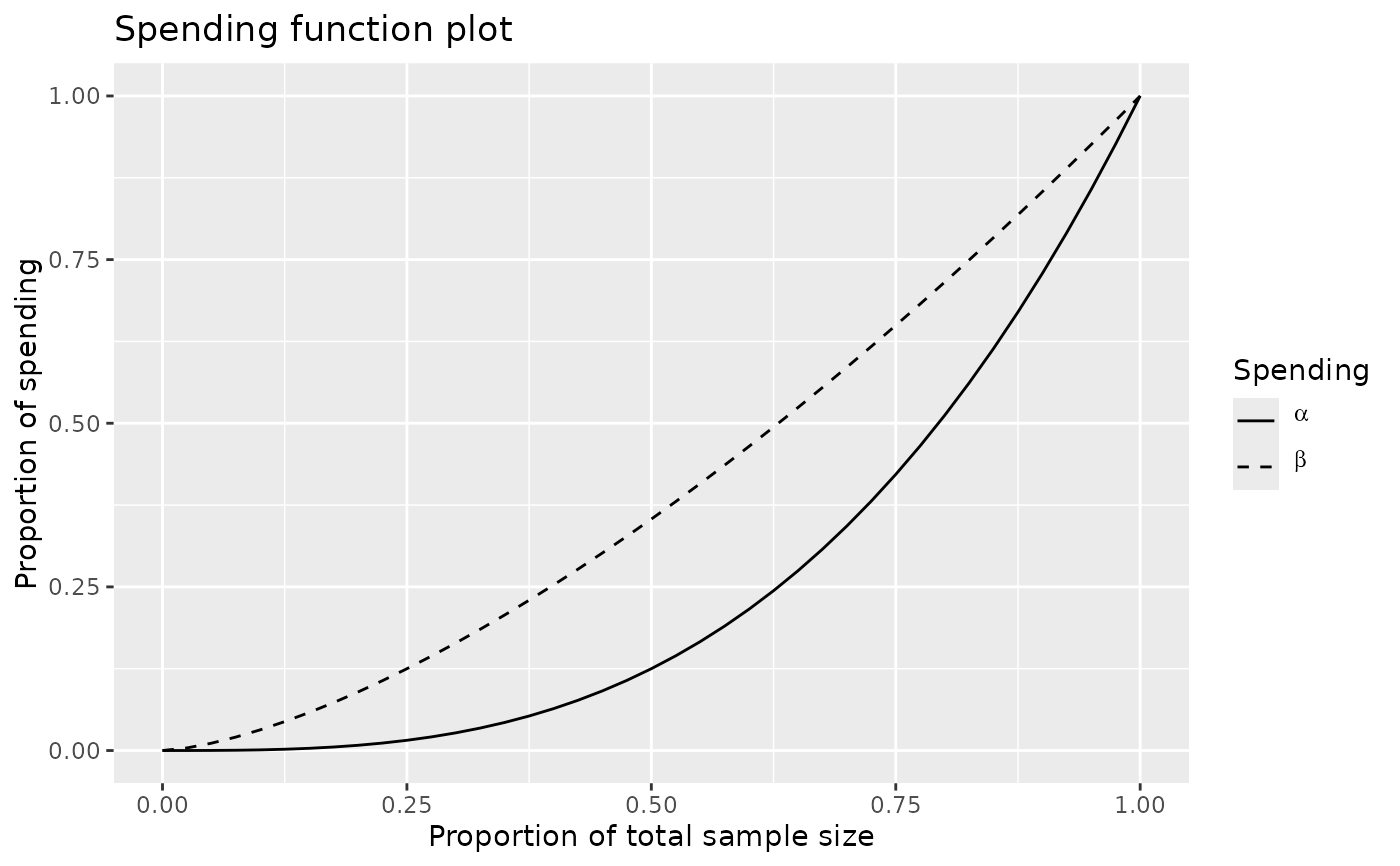
# plot the alpha- and beta-spending functions
plot(x, plottype = 5)


# start by showing how to fit two points with sfLogistic
# plot the spending function using many points to obtain a smooth curve
# note that curve fits the points x=.1,  y=.01 and x=.4,  y=.1
# specified in the 3rd parameter of sfLogistic
t <- 0:100 / 100
plot(t, sfLogistic(1, t, c(.1, .4, .01, .1))$spend,
  xlab = "Proportion of final sample size",
  ylab = "Cumulative Type I error spending",
  main = "Logistic Spending Function Examples",
  type = "l", cex.main = .9
)
lines(t, sfLogistic(1, t, c(.01, .1, .1, .4))$spend, lty = 2)

# now just give a=0 and b=1 as 3rd parameters for sfLogistic
lines(t, sfLogistic(1, t, c(0, 1))$spend, lty = 3)

# try a couple with unconventional shapes again using
# the xy form in the 3rd parameter
lines(t, sfLogistic(1, t, c(.4, .6, .1, .7))$spend, lty = 4)
lines(t, sfLogistic(1, t, c(.1, .7, .4, .6))$spend, lty = 5)
legend(
  x = c(.0, .475), y = c(.76, 1.03), lty = 1:5,
  legend = c(
    "Fit (.1, 01) and (.4, .1)", "Fit (.01, .1) and (.1, .4)",
    "a=0,  b=1", "Fit (.4, .1) and (.6, .7)",
    "Fit (.1, .4) and (.7, .6)"
  )
)


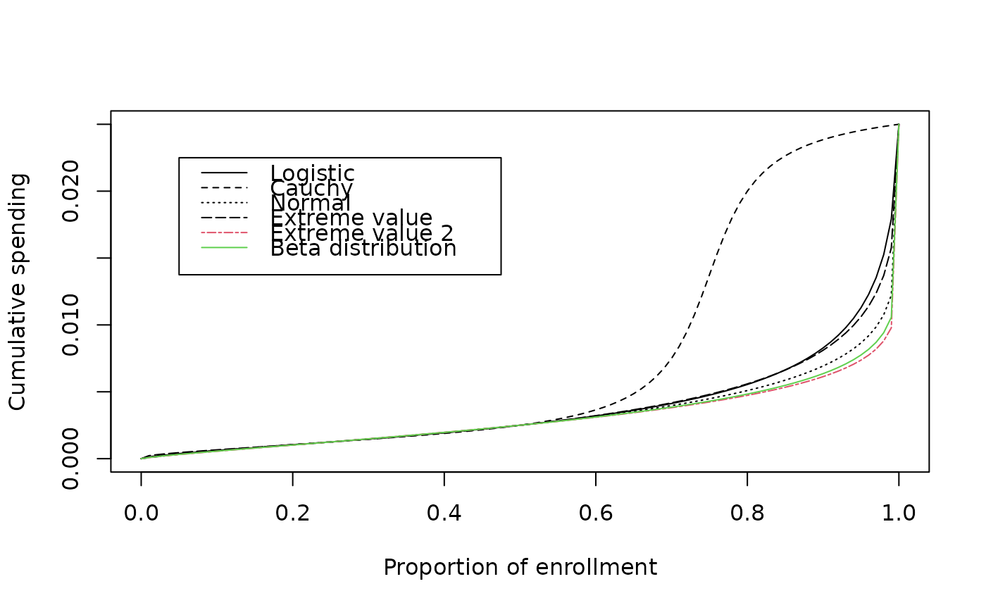
# set up a function to plot comparsons of all
# 2-parameter spending functions
plotsf <- function(alpha, t, param) {
  plot(t, sfCauchy(alpha, t, param)$spend,
    xlab = "Proportion of enrollment",
    ylab = "Cumulative spending", type = "l", lty = 2
  )
  lines(t, sfExtremeValue(alpha, t, param)$spend, lty = 5)
  lines(t, sfLogistic(alpha, t, param)$spend, lty = 1)
  lines(t, sfNormal(alpha, t, param)$spend, lty = 3)
  lines(t, sfExtremeValue2(alpha, t, param)$spend, lty = 6, col = 2)
  lines(t, sfBetaDist(alpha, t, param)$spend, lty = 7, col = 3)
  legend(
    x = c(.05, .475), y = .025 * c(.55, .9),
    lty = c(1, 2, 3, 5, 6, 7),
    col = c(1, 1, 1, 1, 2, 3),
    legend = c(
      "Logistic", "Cauchy", "Normal", "Extreme value",
      "Extreme value 2", "Beta distribution"
    )
  )
}
# do comparison for a design with conservative early spending
# note that Cauchy spending function is quite different
# from the others
param <- c(.25, .5, .05, .1)
plotsf(.025, t, param)