Testing, Confidence Intervals, Sample Size and Power for Comparing Two Binomial Rates

Support is provided for sample size estimation, power, testing, confidence intervals and simulation for fixed sample size trials (that is, not group sequential or adaptive) with two arms and binary outcomes. Both superiority and non-inferiority trials are considered. While all routines default to comparisons of risk-difference, options to base computations on risk-ratio and odds-ratio are also included.

nBinomial() computes sample size or power using the method of Farrington and Manning (1990) for a trial to test the difference between two binomial event rates. The routine can be used for a test of superiority or non-inferiority. For a design that tests for superiority nBinomial() is consistent with the method of Fleiss, Tytun, and Ury (but without the continuity correction) to test for differences between event rates. This routine is consistent with the Hmisc package routines bsamsize and bpower for superiority designs. Vector arguments allow computing sample sizes for multiple scenarios for comparative purposes.

testBinomial() computes a Z- or Chi-square-statistic that compares two binomial event rates using the method of Miettinen and Nurminen (1980). This can be used for superiority or non-inferiority testing. Vector arguments allow easy incorporation into simulation routines for fixed, group sequential and adaptive designs.

ciBinomial() computes confidence intervals for 1) the difference between two rates, 2) the risk-ratio for two rates or 3) the odds-ratio for two rates. This procedure provides inference that is consistent with testBinomial() in that the confidence intervals are produced by inverting the testing procedures in testBinomial(). The Type I error alpha input to ciBinomial is always interpreted as 2-sided.

simBinomial() performs simulations to estimate the power for a Miettinen and Nurminen (1985) test comparing two binomial rates for superiority or non-inferiority. As noted in documentation for bpower.sim() in the HMisc package, by using testBinomial() you can see that the formulas without any continuity correction are quite accurate. In fact, Type I error for a continuity-corrected test is significantly lower (Gordon and Watson, 1996) than the nominal rate. Thus, as a default no continuity corrections are performed.

varBinomial computes blinded estimates of the variance of the estimate of 1) event rate differences, 2) logarithm of the risk ratio, or 3) logarithm of the odds ratio. This is intended for blinded sample size re-estimation for comparative trials with a binary outcome.

Testing is 2-sided when a Chi-square statistic is used and 1-sided when a Z-statistic is used. Thus, these 2 options will produce substantially different results, in general. For non-inferiority, 1-sided testing is appropriate.

You may wish to round sample sizes up using ceiling().

Farrington and Manning (1990) begin with event rates p1 and p2 under the alternative hypothesis and a difference between these rates under the null hypothesis, delta0. From these values, actual rates under the null hypothesis are computed, which are labeled p10 and p20 when outtype=3. The rates p1 and p2 are used to compute a variance for a Z-test comparing rates under the alternative hypothesis, while p10 and p20 are used under the null hypothesis. This computational method is also used to estimate variances in varBinomial() based on the overall event rate observed and the input treatment difference specified in delta0.

Sample size with scale="Difference" produces an error if p1-p2=delta0. Normally, the alternative hypothesis under consideration would be p1-p2-delta0$>0$. However, the alternative can have p1-p2-delta0$<0$.

Usage

ciBinomial(x1, x2, n1, n2, alpha = 0.05, adj = 0, scale = "Difference")

nBinomial(
  p1,
  p2,
  alpha = 0.025,
  beta = 0.1,
  delta0 = 0,
  ratio = 1,
  sided = 1,
  outtype = 1,
  scale = "Difference",
  n = NULL
)

simBinomial(
  p1,
  p2,
  n1,
  n2,
  delta0 = 0,
  nsim = 10000,
  chisq = 0,
  adj = 0,
  scale = "Difference"
)

testBinomial(
  x1,
  x2,
  n1,
  n2,
  delta0 = 0,
  chisq = 0,
  adj = 0,
  scale = "Difference",
  tol = 1e-11
)

varBinomial(x, n, delta0 = 0, ratio = 1, scale = "Difference")

Arguments

x1: Number of “successes” in the control group
x2: Number of “successes” in the experimental group
n1: Number of observations in the control group
n2: Number of observations in the experimental group
alpha: type I error; see sided below to distinguish between 1- and 2-sided tests
adj: With adj=1, the standard variance with a continuity correction is used for a Miettinen and Nurminen test statistic This includes a factor of $n / (n - 1)$ where $n$ is the total sample size. If adj is not 1, this factor is not applied. The default is adj=0 since nominal Type I error is generally conservative with adj=1 (Gordon and Watson, 1996).
scale: “Difference”, “RR”, “OR”; see the scale parameter documentation above and Details. This is a scalar argument.
p1: event rate in group 1 under the alternative hypothesis
p2: event rate in group 2 under the alternative hypothesis
beta: type II error
delta0: A value of 0 (the default) always represents no difference between treatment groups under the null hypothesis. delta0 is interpreted differently depending on the value of the parameter scale. If scale="Difference" (the default), delta0 is the difference in event rates under the null hypothesis (p10 - p20). If scale="RR", delta0 is the logarithm of the relative risk of event rates (p10 / p20) under the null hypothesis. If scale="LNOR", delta0 is the difference in natural logarithm of the odds-ratio under the null hypothesis log(p10 / (1 - p10)) - log(p20 / (1 - p20)).
ratio: sample size ratio for group 2 divided by group 1
sided: 2 for 2-sided test, 1 for 1-sided test
outtype: nBinomial only; 1 (default) returns total sample size; 2 returns a data frame with sample size for each group (n1, n2; if n is not input as NULL, power is returned in Power; 3 returns a data frame with total sample size (n), sample size in each group (n1, n2), Type I error (alpha), 1 or 2 (sided, as input), Type II error (beta), power (Power), null and alternate hypothesis standard deviations (sigma0, sigma1), input event rates (p1, p2), null hypothesis difference in treatment group means (delta0) and null hypothesis event rates (p10, p20).
n: If power is to be computed in nBinomial(), input total trial sample size in n; this may be a vector. This is also the sample size in varBinomial, in which case the argument must be a scalar.
nsim: The number of simulations to be performed in simBinomial()
chisq: An indicator of whether or not a chi-square (as opposed to Z) statistic is to be computed. If delta0=0 (default), the difference in event rates divided by its standard error under the null hypothesis is used. Otherwise, a Miettinen and Nurminen chi-square statistic for a 2 x 2 table is used.
tol: Default should probably be used; this is used to deal with a rounding issue in interim calculations
x: Number of “successes” in the combined control and experimental groups.

Value

testBinomial() and simBinomial() each return a vector of either Chi-square or Z test statistics. These may be compared to an appropriate cutoff point (e.g., qnorm(.975) for normal or qchisq(.95,1) for chi-square).

ciBinomial() returns a data frame with 1 row with a confidence interval; variable names are lower and upper.

varBinomial() returns a vector of (blinded) variance estimates of the difference of event rates (scale="Difference"), logarithm of the odds-ratio (scale="OR") or logarithm of the risk-ratio (scale="RR").

With the default outtype=1, nBinomial() returns a vector of total sample sizes is returned. With outtype=2, nBinomial() returns a data frame containing two vectors n1 and n2 containing sample sizes for groups 1 and 2, respectively; if n is input, this option also returns the power in a third vector, Power. With outtype=3, nBinomial() returns a data frame with the following columns:

n: A vector with total samples size required for each event rate comparison specified
n1: A vector of sample sizes for group 1 for each event rate comparison specified
n2: A vector of sample sizes for group 2 for each event rate comparison specified
alpha: As input
sided: As input
beta: As input; if n is input, this is computed
Power: If n=NULL on input, this is 1-beta; otherwise, the power is computed for each sample size input
sigma0: A vector containing the standard deviation of the treatment effect difference under the null hypothesis times sqrt(n) when scale="Difference" or scale="OR"; when scale="RR", this is the standard deviation time sqrt(n) for the numerator of the Farrington-Manning test statistic x1-exp(delta0)*x2.
sigma1: A vector containing the values as sigma0, in this case estimated under the alternative hypothesis.
p1: As input
p2: As input
p10: group 1 event rate used for null hypothesis
p20: group 2 event rate used for null hypothesis

References

Farrington, CP and Manning, G (1990), Test statistics and sample size formulae for comparative binomial trials with null hypothesis of non-zero risk difference or non-unity relative risk. Statistics in Medicine; 9: 1447-1454.

Fleiss, JL, Tytun, A and Ury (1980), A simple approximation for calculating sample sizes for comparing independent proportions. Biometrics;36:343-346.

Gordon, I and Watson R (1985), The myth of continuity-corrected sample size formulae. Biometrics; 52: 71-76.

Miettinen, O and Nurminen, M (1985), Comparative analysis of two rates. Statistics in Medicine; 4 : 213-226.

Author

Keaven Anderson keaven_anderson@merck.com

Examples


# Compute z-test test statistic comparing 39/500 to 13/500
# use continuity correction in variance
x <- testBinomial(x1 = 39, x2 = 13, n1 = 500, n2 = 500, adj = 1)
x
#> [1] 3.701266
pnorm(x, lower.tail = FALSE)
#> [1] 0.0001072634

# Compute with unadjusted variance
x0 <- testBinomial(x1 = 39, x2 = 23, n1 = 500, n2 = 500)
x0
#> [1] 2.098083
pnorm(x0, lower.tail = FALSE)
#> [1] 0.0179489

# Perform 50k simulations to test validity of the above
# asymptotic p-values
# (you may want to perform more to reduce standard error of estimate)
sum(as.double(x0) <=
  simBinomial(p1 = .078, p2 = .078, n1 = 500, n2 = 500, nsim = 10000)) / 10000
#> [1] 0.0173
sum(as.double(x0) <=
  simBinomial(p1 = .052, p2 = .052, n1 = 500, n2 = 500, nsim = 10000)) / 10000
#> [1] 0.0179

# Perform a non-inferiority test to see if p2=400 / 500 is within 5% of
# p1=410 / 500 use a z-statistic with unadjusted variance
x <- testBinomial(x1 = 410, x2 = 400, n1 = 500, n2 = 500, delta0 = -.05)
x
#> [1] 2.807617
pnorm(x, lower.tail = FALSE)
#> [1] 0.002495478

# since chi-square tests equivalence (a 2-sided test) rather than
# non-inferiority (a 1-sided test),
# the result is quite different
pchisq(testBinomial(
  x1 = 410, x2 = 400, n1 = 500, n2 = 500, delta0 = -.05,
  chisq = 1, adj = 1
), 1, lower.tail = FALSE)
#> [1] 0.005012758

# now simulate the z-statistic witthout continuity corrected variance
sum(qnorm(.975) <=
  simBinomial(p1 = .8, p2 = .8, n1 = 500, n2 = 500, nsim = 100000)) / 100000
#> [1] 0.02497

# compute a sample size to show non-inferiority
# with 5% margin, 90% power
nBinomial(p1 = .2, p2 = .2, delta0 = .05, alpha = .025, sided = 1, beta = .1)
#> [1] 2697.607

# assuming a slight advantage in the experimental group lowers
# sample size requirement
nBinomial(p1 = .2, p2 = .19, delta0 = .05, alpha = .025, sided = 1, beta = .1)
#> [1] 4131.9

# compute a sample size for comparing 15% vs 10% event rates
# with 1 to 2 randomization
nBinomial(p1 = .15, p2 = .1, beta = .2, ratio = 2, alpha = .05)
#> [1] 1191.041

# now look at total sample size using 1-1 randomization
n <- nBinomial(p1 = .15, p2 = .1, beta = .2, alpha = .05)
n
#> [1] 1079.853
# check if inputing sample size returns the desired power
nBinomial(p1 = .15, p2 = .1, beta = .2, alpha = .05, n = n)
#> [1] 0.8

# re-do with alternate output types
nBinomial(p1 = .15, p2 = .1, beta = .2, alpha = .05, outtype = 2)
#>         n1       n2
#> 1 539.9264 539.9264
nBinomial(p1 = .15, p2 = .1, beta = .2, alpha = .05, outtype = 3)
#>          n       n1       n2 alpha sided beta Power    sigma0    sigma1   p1
#> 1 1079.853 539.9264 539.9264  0.05     1  0.2   0.8 0.6614378 0.6595453 0.15
#>    p2 delta0   p10   p20
#> 1 0.1      0 0.125 0.125

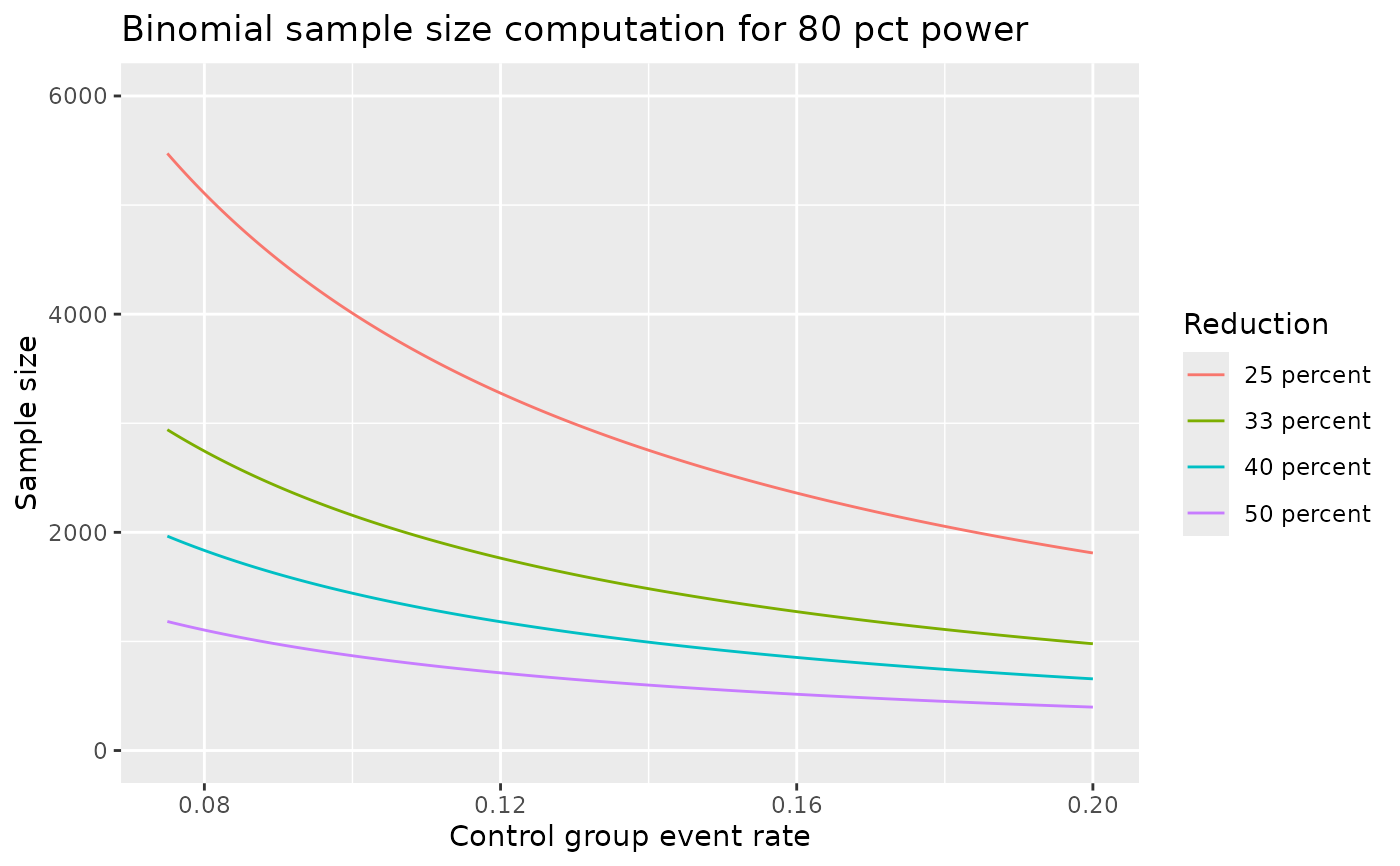
# look at power plot under different control event rate and
# relative risk reductions
library(dplyr)
#> 
#> Attaching package: ‘dplyr’
#> The following objects are masked from ‘package:stats’:
#> 
#>     filter, lag
#> The following objects are masked from ‘package:base’:
#> 
#>     intersect, setdiff, setequal, union
library(ggplot2)
p1 <- seq(.075, .2, .000625)
len <- length(p1)
p2 <- c(p1 * .75, p1 * 2/3, p1 * .6, p1 * .5)
Reduction <- c(rep("25 percent", len), rep("33 percent", len), 
               rep("40 percent", len), rep("50 percent", len))
df <- tibble(p1 = rep(p1, 4), p2, Reduction) %>% 
  mutate(`Sample size` = nBinomial(p1, p2, beta = .2, alpha = .025, sided = 1))
ggplot(df, aes(x = p1, y = `Sample size`, col = Reduction)) + 
  geom_line() + 
  xlab("Control group event rate") +
  ylim(0,6000) +
  ggtitle("Binomial sample size computation for 80 pct power")


# compute blinded estimate of treatment effect difference
x1 <- rbinom(n = 1, size = 100, p = .2)
x2 <- rbinom(n = 1, size = 200, p = .1)
# blinded estimate of risk difference variance
varBinomial(x = x1 + x2, n = 300, ratio = 2, delta0 = 0)
#> [1] 0.0012285
# blinded estimate of log-risk-ratio variance
varBinomial(x = x1 + x2, n = 300, ratio = 2, delta0 = 0, scale = "RR")
#> [1] 0.1516667
# blinded estimate of log-odds-ratio variance
varBinomial(x = x1 + x2, n = 300, ratio = 2, delta0 = 0, scale = "OR")
#> [1] 0.1831502