Diagnosing Blinded Information Calculation Issues
Source:vignettes/blinded-info-diagnostics.Rmd
blinded-info-diagnostics.RmdOverview
This vignette examines two diagnostic datasets where direct maximum-likelihood blinded information estimation produced extreme values during development. Understanding these edge cases explains why the current implementation records estimator fallback paths and uses method-of-moments (MoM) estimates when the pooled negative binomial fit is unreliable.
We examine two scenarios:
-
Near-zero blinded information: Cases where direct
pooled ML estimation can drive
blinded_infoclose to 0 despite reasonableunblinded_info - Historical extreme high blinded information: A case where the raw pooled ML fit produced an astronomical information estimate before the MoM fallback was added
Both scenarios arise from instability in negative binomial model fitting on blinded (pooled) data.
Dataset 1: Near-Zero Blinded Information
This dataset was identified from simulations where
blinded_info = 0.02 while
unblinded_info = 48.6 — a ratio of 0.0004.
# Load the problematic dataset
# Try package location first, fall back to relative path for development
data_path <- system.file("extdata", "problematic_dataset.rds", package = "gsDesignNB")
if (data_path == "") {
  # During development, find the package root
  data_path <- file.path("..", "inst", "extdata", "problematic_dataset.rds")
}
cut_data <- readRDS(data_path)
dt <- as.data.table(cut_data)
Event Counts Summary
# Overall summary
cat("Total subjects:", nrow(dt), "\n")
#> Total subjects: 360
cat("Total events:", sum(dt$events), "\n")
#> Total events: 209
cat("Mean events per subject:", round(mean(dt$events), 3), "\n")
#> Mean events per subject: 0.581
cat("Variance of events:", round(var(dt$events), 3), "\n")
#> Variance of events: 0.79
cat("Variance/Mean ratio:", round(var(dt$events) / mean(dt$events), 3), "\n")
#> Variance/Mean ratio: 1.361

# By treatment
dt[, .(
  n = .N,
  total_events = sum(events),
  mean_events = round(mean(events), 3),
  var_events = round(var(events), 3),
  pct_zero_events = round(100 * mean(events == 0), 1)
), by = treatment]
#>       treatment     n total_events mean_events var_events pct_zero_events
#>          <char> <int>        <int>       <num>      <num>           <num>
#> 1:      control   180          132       0.733      0.979            55.6
#> 2: experimental   180           77       0.428      0.559            68.3
Event Distribution
# Event count distribution
event_dist <- dt[, .(count = .N), by = .(treatment, events)]
event_dist[order(treatment, events)]
#>        treatment events count
#>           <char>  <int> <int>
#>  1:      control      0   100
#>  2:      control      1    45
#>  3:      control      2    19
#>  4:      control      3    15
#>  5:      control      4     1
#>  6: experimental      0   123
#>  7: experimental      1    44
#>  8: experimental      2     7
#>  9: experimental      3     5
#> 10: experimental      4     1
A key observation is the high proportion of subjects with zero events, particularly in the experimental arm.
Event Rates by Patient
We calculate the event rate as events divided by follow-up duration
(tte).
dt[, event_rate := events / tte]

# Summary of event rates
dt[, .(
  n = .N,
  mean_rate = round(mean(event_rate), 4),
  median_rate = round(median(event_rate), 4),
  sd_rate = round(sd(event_rate), 4),
  pct_zero_rate = round(100 * mean(event_rate == 0), 1)
), by = treatment]
#>       treatment     n mean_rate median_rate sd_rate pct_zero_rate
#>          <char> <int>     <num>       <num>   <num>         <num>
#> 1:      control   180    0.1624           0  0.2847          55.6
#> 2: experimental   180    1.2725           0 15.8474          68.3
Violin Plot of Event Rates
# Add overall group for comparison
dt_plot <- rbind(
  dt[, .(treatment = treatment, event_rate = event_rate)],
  dt[, .(treatment = "Overall (Pooled)", event_rate = event_rate)]
)

ggplot(dt_plot, aes(x = treatment, y = event_rate, fill = treatment)) +
  geom_violin(alpha = 0.7, scale = "width") +
  geom_boxplot(width = 0.1, fill = "white", alpha = 0.8) +
  labs(
    title = "Distribution of Patient-Level Event Rates",
    subtitle = "Dataset with Near-Zero Blinded Information",
    x = "Treatment Group",
    y = "Event Rate (events / follow-up time)"
  ) +
  theme_minimal() +
  theme(legend.position = "none") +
  scale_fill_brewer(palette = "Set2")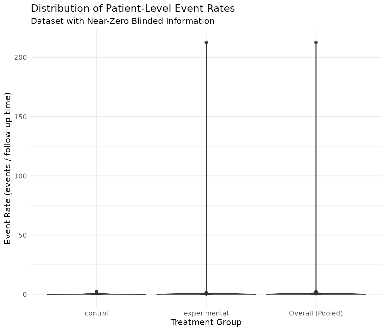
The violin plot shows that many subjects have zero event rates, creating a spike at zero. The control arm has higher event rates than the experimental arm, as expected given the simulation parameters.
What Happened with the Information Calculations
# Blinded information calculation
blinded_res <- calculate_blinded_info(
  cut_data,
  ratio = 1,
  lambda1_planning = 1.5/12,
  lambda2_planning = 1.0/12
)

cat("Blinded Information Results:\n")
#> Blinded Information Results:
cat("  blinded_info:", blinded_res$blinded_info, "\n")
#>   blinded_info: 0.0201878
cat("  dispersion_blinded:", blinded_res$dispersion_blinded, "\n")
#>   dispersion_blinded: 4454.477
cat("  lambda_blinded:", blinded_res$lambda_blinded, "\n")
#>   lambda_blinded: 0.6791599

# Unblinded calculation via mutze_test
mutze_res <- mutze_test(cut_data)

cat("\nUnblinded (Mutze Test) Results:\n")
#>
#> Unblinded (Mutze Test) Results:
cat("  method:", mutze_res$method, "\n")
#>   method: Negative binomial Wald (MoM fallback, extreme overdispersion)
cat("  SE:", round(mutze_res$se, 4), "\n")
#>   SE: 0.1553
cat("  unblinded_info (1/SE^2):", round(1/mutze_res$se^2, 2), "\n")
#>   unblinded_info (1/SE^2): 41.47
cat("  dispersion:", mutze_res$dispersion, "\n")
#>   dispersion: 4.088287
Root Cause Analysis
The issue stems from the blinded glm.nb fit:
df <- as.data.frame(cut_data)
df <- df[df$tte > 0, ]

# Blinded fit (no treatment effect)
fit_blinded <- suppressWarnings(MASS::glm.nb(events ~ 1 + offset(log(tte)), data = df))

cat("Blinded glm.nb fit:\n")
#> Blinded glm.nb fit:
cat("  theta:", fit_blinded$theta, "\n")
#>   theta: 0.0002244933
cat("  1/theta (dispersion):", 1/fit_blinded$theta, "\n")
#>   1/theta (dispersion): 4454.477

# Unblinded fit (with treatment effect)
fit_unblinded <- suppressWarnings(MASS::glm.nb(events ~ treatment + offset(log(tte)), data = df))

cat("\nUnblinded glm.nb fit:\n")
#>
#> Unblinded glm.nb fit:
cat("  theta:", fit_unblinded$theta, "\n")
#>   theta: 0.000138869
cat("  1/theta (dispersion):", 1/fit_unblinded$theta, "\n")
#>   1/theta (dispersion): 7201.033
The Problem: The blinded glm.nb fit
returns an extremely small theta (≈ 0.0002), which
translates to dispersion_blinded = 1/theta ≈ 4454.
The blinded information formula is: \[w_j = p_j \sum_i \frac{\mu_{ij}}{1 + k \cdot \mu_{ij}}\]
where \(k\) is the dispersion and \(\mu_{ij} = \lambda_j \cdot t_i\).
When \(k\) is very large (4454), the denominator becomes huge: \[1 + 4454 \times 0.5 \approx 2228\]
This makes \(w_j\) approximately 2000 times smaller than it should be, causing the information to collapse to near-zero.
Method of Moments Comparison
Here we compare the problematic MLE estimate with the Method of Moments (MoM) estimator.
# Calculate MoM estimates
mom_res <- estimate_nb_mom(df)

cat("Method of Moments (Blinded) Estimation:\n")
#> Method of Moments (Blinded) Estimation:
cat("  Lambda (Rate):", round(mom_res$lambda, 4), "\n")
#>   Lambda (Rate): 0.1169
cat("  Dispersion (k):", round(mom_res$dispersion, 4), "\n")
#>   Dispersion (k): 0.3292
The MoM estimator produces a much more reasonable dispersion estimate compared to the MLE’s 4454. This suggests the MoM approach is more robust to this specific data distribution where the “blinded” assumption (single rate) is violated by the treatment effect.
Dataset 2: Extreme High Blinded Information
This dataset was originally identified from a group-sequential
simulation where the direct pooled ML calculation produced
blinded_info = 1.84 × 10^38, an astronomically large value
indicating numerical overflow. The current
calculate_blinded_info() implementation falls back to MoM
for this dataset, so the helper output below should be finite.
# Load the historical extreme-high dataset
data_path_2 <- system.file("extdata", "extreme_high_dataset.rds", package = "gsDesignNB")
if (data_path_2 == "") {
  data_path_2 <- file.path("..", "inst", "extdata", "extreme_high_dataset.rds")
}
cut_data_2 <- readRDS(data_path_2)
dt2 <- as.data.table(cut_data_2)
Event Counts Summary
# Overall summary
cat("Total subjects:", nrow(dt2), "\n")
#> Total subjects: 313
cat("Total events:", sum(dt2$events), "\n")
#> Total events: 116
cat("Mean events per subject:", round(mean(dt2$events), 3), "\n")
#> Mean events per subject: 0.371
cat("Variance of events:", round(var(dt2$events), 3), "\n")
#> Variance of events: 0.458
cat("Variance/Mean ratio:", round(var(dt2$events) / mean(dt2$events), 3), "\n")
#> Variance/Mean ratio: 1.237

# By treatment
dt2[, .(
  n = .N,
  total_events = sum(events),
  mean_events = round(mean(events), 3),
  var_events = round(var(events), 3),
  pct_zero_events = round(100 * mean(events == 0), 1)
), by = treatment]
#>       treatment     n total_events mean_events var_events pct_zero_events
#>          <char> <int>        <int>       <num>      <num>           <num>
#> 1: Experimental   156           42       0.269      0.314            78.2
#> 2:      Control   157           74       0.471      0.584            66.2
What Happened with the Information Calculations
# Blinded information calculation
blinded_res_2 <- calculate_blinded_info(
  cut_data_2,
  ratio = 1,
  lambda1_planning = 1.5/12,
  lambda2_planning = 1.0/12
)
#> Warning: Blinded ML NB fit did not converge; falling back to method-of-moments
#> (lambda = 0.09262, k = 0.4033).

cat("Blinded Information Results:\n")
#> Blinded Information Results:
cat("  blinded_info:", format(blinded_res_2$blinded_info, scientific = TRUE), "\n")
#>   blinded_info: 2.312778e+01
cat("  dispersion_blinded:", format(blinded_res_2$dispersion_blinded, scientific = TRUE), "\n")
#>   dispersion_blinded: 4.03252e-01
cat("  lambda_blinded:", round(blinded_res_2$lambda_blinded, 4), "\n")
#>   lambda_blinded: 0.0926

# Unblinded calculation via mutze_test
mutze_res_2 <- mutze_test(cut_data_2)

cat("\nUnblinded (Mutze Test) Results:\n")
#>
#> Unblinded (Mutze Test) Results:
cat("  method:", mutze_res_2$method, "\n")
#>   method: Negative binomial Wald (MoM fallback, ML non-convergent)
cat("  SE:", round(mutze_res_2$se, 4), "\n")
#>   SE: 0.2078
cat("  unblinded_info (1/SE^2):", round(1/mutze_res_2$se^2, 2), "\n")
#>   unblinded_info (1/SE^2): 23.16
cat("  dispersion:", mutze_res_2$dispersion, "\n")
#>   dispersion: 3.110089
Root Cause Analysis
df2 <- as.data.frame(cut_data_2)
df2 <- df2[df2$tte > 0, ]

# Blinded fit (no treatment effect)
fit_blinded_2 <- tryCatch(
  suppressWarnings(MASS::glm.nb(events ~ 1 + offset(log(tte)), data = df2)),
  error = function(e) NULL
)

if (!is.null(fit_blinded_2)) {
  cat("Blinded glm.nb fit:\n")
  cat("  theta:", format(fit_blinded_2$theta, scientific = TRUE), "\n")
  cat("  1/theta (dispersion):", format(1/fit_blinded_2$theta, scientific = TRUE), "\n")
} else {
  cat("Blinded glm.nb fit FAILED\n")
}
#> Blinded glm.nb fit:
#>   theta: 1.70209e+41
#>   1/theta (dispersion): 5.875129e-42

# Unblinded fit (with treatment effect)
fit_unblinded_2 <- tryCatch(
  suppressWarnings(MASS::glm.nb(events ~ treatment + offset(log(tte)), data = df2)),
  error = function(e) NULL
)

if (!is.null(fit_unblinded_2)) {
  cat("\nUnblinded glm.nb fit:\n")
  cat("  theta:", round(fit_unblinded_2$theta, 4), "\n")
  cat("  1/theta (dispersion):", round(1/fit_unblinded_2$theta, 4), "\n")
} else {
  cat("\nUnblinded glm.nb fit FAILED - this explains the Poisson fallback\n")
}
#>
#> Unblinded glm.nb fit FAILED - this explains the Poisson fallback
The Problem: The blinded glm.nb returns
an astronomically large theta (≈ 1.7 × 10^41), which
translates to dispersion_blinded ≈ 5.9 × 10^-42 —
essentially zero.
The information formula depends on: \[w_j = p_j \sum_i \frac{\mu_{ij}}{1 + k \cdot \mu_{ij}}\]
When \(k \to 0\): \[w_j \approx p_j \sum_i \mu_{ij}\]
This makes \(w_j\) very large, and since variance = \(1/w_1 + 1/w_2\), the variance approaches zero, causing information = 1/variance to overflow to infinity.
Method of Moments Comparison
Again, we compare with the Method of Moments (MoM) estimator.
# Calculate MoM estimates
mom_res_2 <- estimate_nb_mom(df2)

cat("Method of Moments (Blinded) Estimation:\n")
#> Method of Moments (Blinded) Estimation:
cat("  Lambda (Rate):", round(mom_res_2$lambda, 4), "\n")
#>   Lambda (Rate): 0.0926
cat("  Dispersion (k):", mom_res_2$dispersion, "\n")
#>   Dispersion (k): 0.403252
In this case, the MoM estimator returns a finite dispersion estimate, avoiding the numerical instability of the infinite-theta ML path.
Why the Mutze Test Falls Back to Poisson
Note that mutze_test reports
dispersion = Inf and uses the “Poisson Wald (fallback)”
method. This happens because glm.nb with the treatment
effect also struggles with this dataset — the theta estimate becomes
unstable, and the function falls back to a simpler Poisson model.
Summary of Issues
| Issue | Current helper behavior | Historical / raw ML cause |
|---|---|---|
| Near-zero | ML path can still produce very small blinded information; compare against unblinded and MoM paths | Extremely large pooled dispersion estimate |
| Historical near-infinite | Current helper uses MoM fallback and returns finite information | Non-convergent or boundary pooled ML fit with effectively zero dispersion |
Both issues arise from instability in glm.nb when
fitting to pooled (blinded) data. The pooling can create artificial
variance patterns that do not represent the true data-generating
process.
Recommendations
Inspect extreme ML paths: Compare ML and MoM information estimates when pooled ML produces boundary-like dispersion estimates.
Use assumed dispersion: Consider using the planned/assumed dispersion from the design rather than estimating from blinded data
Add sanity checks: Flag cases where blinded info differs from unblinded info by more than a factor of 2-3
Fallback to unblinded: When blinded estimation produces extreme values, fall back to the unblinded information
Use Method of Moments (MoM): The analysis above demonstrates that a simple Method of Moments estimator is more robust than
glm.nbfor blinded parameter estimation in these edge cases. It provides reasonable dispersion estimates when the blinded MLE fails or returns boundary-like values.
sessionInfo()
#> R version 4.6.1 (2026-06-24)
#> Platform: x86_64-pc-linux-gnu
#> Running under: Ubuntu 24.04.4 LTS
#>
#> Matrix products: default
#> BLAS:   /usr/lib/x86_64-linux-gnu/openblas-pthread/libblas.so.3
#> LAPACK: /usr/lib/x86_64-linux-gnu/openblas-pthread/libopenblasp-r0.3.26.so;  LAPACK version 3.12.0
#>
#> locale:
#>  [1] LC_CTYPE=C.UTF-8       LC_NUMERIC=C           LC_TIME=C.UTF-8
#>  [4] LC_COLLATE=C.UTF-8     LC_MONETARY=C.UTF-8    LC_MESSAGES=C.UTF-8
#>  [7] LC_PAPER=C.UTF-8       LC_NAME=C              LC_ADDRESS=C
#> [10] LC_TELEPHONE=C         LC_MEASUREMENT=C.UTF-8 LC_IDENTIFICATION=C
#>
#> time zone: UTC
#> tzcode source: system (glibc)
#>
#> attached base packages:
#> [1] stats     graphics  grDevices utils     datasets  methods   base
#>
#> other attached packages:
#> [1] MASS_7.3-65       ggplot2_4.0.3     data.table_1.18.4 gsDesignNB_0.3.2
#>
#> loaded via a namespace (and not attached):
#>  [1] gt_1.3.0            sass_0.4.10         future_1.70.0
#>  [4] generics_0.1.4      tidyr_1.3.2         xml2_1.6.0
#>  [7] r2rtf_1.3.1         lattice_0.22-9      listenv_1.0.0
#> [10] digest_0.6.39       magrittr_2.0.5      evaluate_1.0.5
#> [13] grid_4.6.1          RColorBrewer_1.1-3  iterators_1.0.14
#> [16] mvtnorm_1.4-1       fastmap_1.2.0       Matrix_1.7-5
#> [19] foreach_1.5.2       simtrial_1.0.2      jsonlite_2.0.0
#> [22] survival_3.8-6      purrr_1.2.2         scales_1.4.0
#> [25] codetools_0.2-20    textshaping_1.0.5   jquerylib_0.1.4
#> [28] cli_3.6.6           rlang_1.3.0         parallelly_1.48.0
#> [31] future.apply_1.20.2 splines_4.6.1       withr_3.0.3
#> [34] cachem_1.1.0        yaml_2.3.12         gsDesign_3.10.0
#> [37] otel_0.2.0          tools_4.6.1         parallel_4.6.1
#> [40] doFuture_1.2.2      dplyr_1.2.1         globals_0.19.1
#> [43] vctrs_0.7.3         R6_2.6.1            lifecycle_1.0.5
#> [46] fs_2.1.0            htmlwidgets_1.6.4   ragg_1.5.2
#> [49] pkgconfig_2.0.3     desc_1.4.3          pkgdown_2.2.1
#> [52] pillar_1.11.1       bslib_0.11.0        gtable_0.3.6
#> [55] glue_1.8.1          Rcpp_1.1.2          systemfonts_1.3.2
#> [58] xfun_0.60           tibble_3.3.1        tidyselect_1.2.1
#> [61] knitr_1.51          farver_2.1.2        xtable_1.8-8
#> [64] htmltools_0.5.9     labeling_0.4.3      rmarkdown_2.31
#> [67] compiler_4.6.1      S7_0.2.2