Group sequential design and simulation • gsDesignNB

library(gsDesign)
library(gsDesignNB)
library(data.table)
library(ggplot2)
library(gt)

This vignette demonstrates how to create a group sequential design for negative binomial outcomes using gsNBCalendar() and simulate the design to confirm design operating characteristics using nb_sim().

Trial design parameters

We design a trial with the following characteristics:

Enrollment: 12 months with a constant rate
Trial Duration: 24 months
Analyses:
- Interim 1: 10 months
- Interim 2: 18 months
- Final: 24 months
Event Rates:
- Control: 0.125 events per month (1.5 per year)
- Experimental: 0.0833 events per month (1.0 per year; rate ratio = 0.67)
Dispersion: 0.5
Power: 90% (beta = 0.1)
Alpha: 0.025 (one-sided) # event gap: 20 days # dropout rate: 5% at 1 year # max followup: 12 months

Sample size calculation

First, we calculate the required sample size for a fixed design using the Zhu and Lakkis method:

# Sample size calculation
# Enrollment: constant rate over 12 months
# Trial duration: 24 months
event_gap_val <- 20 / 30.4375 # Minimum gap between events is 20 days (approx)

nb_ss <- sample_size_nbinom(
  lambda1 = 1.5 / 12, # Control event rate (per month)
  lambda2 = 1.0 / 12, # Experimental event rate (per month)
  dispersion = 0.5, # Overdispersion parameter
  power = 0.9, # 90% power
  alpha = 0.025, # One-sided alpha
  accrual_rate = 1, # This will be scaled to achieve the target power
  accrual_duration = 12, # 12 months enrollment
  trial_duration = 24, # 24 months trial
  max_followup = 12, # 12 months of follow-up per patient
  dropout_rate = -log(0.95) / 12, # 5% dropout rate at 1 year
  event_gap = event_gap_val,
  method = "zhu" # Zhu and Lakkis sample size method
)

# Print key results
message("Fixed design")
#> Fixed design
nb_ss
#> Sample size for negative binomial outcome
#> ==========================================
#> 
#> Method:          zhu
#> Sample size:     n1 = 182, n2 = 182, total = 364
#> Expected events: 414.1 (n1: 245.9, n2: 168.2)
#> Power: 90%, Alpha: 0.025 (1-sided)
#> Rates: control = 0.1250, treatment = 0.0833 (RR = 0.6667)
#> Dispersion: 0.5000, Avg exposure (calendar): 11.70
#> Avg exposure (at-risk): n1 = 10.81, n2 = 11.09
#> Event gap: 0.66
#> Dropout rate: 0.0043
#> Accrual: 12.0, Trial duration: 24.0
#> Max follow-up: 12.0

Group sequential design

Now we convert this a group sequential design with 3 analyses after 10, 18 and 24 months. Note that the final analysis time must be the same as for the fixed design. The relative enrollment rates will be increased to increase the sample size as with standard group sequential design theory. We specify usTime = c(0.1, 0.18, 1) which along with the sfLinear() spending function will spend 10%, 18% and 100% of the cumulative $\alpha$ at the 3 planned analyses regardless of the observed statistical information at each analysis.

# Analysis times (in months)
analysis_times <- c(10, 18, 24)

# Create group sequential design with integer sample sizes
gs_nb <- gsNBCalendar(
  x = nb_ss, # Input fixed design for negative binomial
  k = 3, # 3 analyses
  test.type = 4, # Two-sided asymmetric, non-binding futility
  sfu = sfLinear, # Linear spending function for upper bound
  sfupar = c(.5, .5), # Identity function
  sfl = sfHSD, # HSD spending for lower bound
  sflpar = -8, # Conservative futility bound
  usTime = c(.1, .18, 1), # Upper spending timing
  lsTime = NULL, # Spending based on information
  analysis_times = analysis_times # Calendar times in months
) |> gsDesignNB::toInteger() # Round to integer sample size

Textual group sequential design summary:

summary(gs_nb)
#> Asymmetric two-sided with non-binding futility bound group sequential design
#> for negative binomial outcomes, 3 analyses, total sample size 370.0, 90 percent
#> power, 2.5 percent (1-sided) Type I error. Control rate 0.1250, treatment rate
#> 0.0833, risk ratio 0.6667, dispersion 0.5000. Accrual duration 12.0, trial
#> duration 24.0, max follow-up 12.0, event gap 0.66, dropout rate 0.0043, average
#> exposure (calendar) 11.70, (at-risk n1=10.81, n2=11.09). Randomization ratio
#> 1:1. Upper spending: Piecewise linear (line points = 0.5) Lower spending:
#> Hwang-Shih-DeCani (gamma = -8)
#> Asymmetric two-sided with non-binding futility bound group sequential design
#> for negative binomial outcomes, 3 analyses, total sample size 370.0, 90 percent
#> power, 2.5 percent (1-sided) Type I error. Control rate 0.1250, treatment rate
#> 0.0833, risk ratio 0.6667, dispersion 0.5000. Accrual duration 12.0, trial
#> duration 24.0, max follow-up 12.0, event gap 0.66, dropout rate 0.0043, average
#> exposure (calendar) 11.70, (at-risk n1=10.81, n2=11.09). Randomization ratio
#> 1:1. Upper spending: Piecewise linear (line points = 0.5) Lower spending:
#> Hwang-Shih-DeCani (gamma = -8)

Tabular summary:

gs_nb |>
  gsDesign::gsBoundSummary(
    deltaname = "RR",
    logdelta = TRUE,
    Nname = "Information",
    timename = "Month",
    digits = 4,
    ddigits = 2
  ) |>
  gt() |>
  tab_header(
    title = "Group Sequential Design Bounds for Negative Binomial Outcome",
    subtitle = paste0(
      "N = ", ceiling(gs_nb$n_total[gs_nb$k]),
      ", Expected events = ", round(gs_nb$nb_design$total_events, 1)
    )
  )

Analysis	Value	Efficacy	Futility
Group Sequential Design Bounds for Negative Binomial Outcome
N = 370, Expected events = 414.1
IA 1: 35%	Z	2.8070	-1.1032
Information: 28.96	p (1-sided)	0.0025	0.8650
Month: 10	~RR at bound	0.5931	1.2279
	P(Cross) if RR=1	0.0025	0.1350
	P(Cross) if RR=0.67	0.2649	0.0005
IA 2: 79%	Z	2.8191	1.1884
Information: 65.47	p (1-sided)	0.0024	0.1173
Month: 18	~RR at bound	0.7054	0.8632
	P(Cross) if RR=1	0.0045	0.8826
	P(Cross) if RR=0.67	0.6910	0.0186
Final	Z	1.9875	1.9875
Information: 82.89	p (1-sided)	0.0234	0.0234
Month: 24	~RR at bound	0.8036	0.8036
	P(Cross) if RR=1	0.0240	0.9760
	P(Cross) if RR=0.67	0.9524	0.0476

Simulation study

We now simulate 50 trials to evaluate the power of the group sequential design assuming design parameters above are correct.

Simulation setup

set.seed(42)
n_sims <- 50

# Enrollment rate (patients per month) to achieve target sample size
n_target <- ceiling(nb_ss$n_total)
enroll_rate_val <- n_target / 12 # All enrolled in 12 months

# Define enrollment
enroll_rate <- data.frame(
  rate = enroll_rate_val,
  duration = 12 # 12 months enrollment
)

# Define failure rates (with dispersion)
fail_rate <- data.frame(
  treatment = c("Control", "Experimental"),
  rate = c(1.5 / 12, 1.0 / 12),
  dispersion = c(0.5, 0.5)
)

# Dropout rate (5% at 1 year)
dropout_rate_val <- -log(0.95)
dropout_rate <- data.frame(
  treatment = c("Control", "Experimental"),
  rate = c(dropout_rate_val, dropout_rate_val),
  duration = c(100, 100) # Long duration
)

# Maximum follow-up (trial duration from enrollment start)
max_followup <- 12 # 12 months to match design

Run simulations

# Storage for results
results <- vector("list", n_sims)

for (sim in 1:n_sims) {
  # Simulate trial data
  sim_data <- nb_sim(
    enroll_rate = enroll_rate,
    fail_rate = fail_rate,
    dropout_rate = dropout_rate,
    max_followup = max_followup,
    n = n_target
  )

  # Analyze at each interim
  sim_results <- data.frame(
    sim = sim,
    analysis = 1:3,
    analysis_time = analysis_times,
    n_enrolled = NA_integer_,
    events_ctrl = NA_integer_,
    events_exp = NA_integer_,
    events_total = NA_integer_,
    exposure_ctrl = NA_real_,
    exposure_exp = NA_real_,
    blinded_info = NA_real_,
    unblinded_info = NA_real_,
    z_stat = NA_real_,
    p_value = NA_real_,
    cross_upper = NA,
    cross_lower = NA
  )

  stopped <- FALSE

  for (k in 1:3) {
    if (stopped) {
      # Trial already stopped at earlier analysis
      sim_results$cross_upper[k] <- FALSE
      sim_results$cross_lower[k] <- FALSE
      next
    }

    # Cut data at analysis time
    cut_time <- analysis_times[k]
    cut_data <- cut_data_by_date(sim_data, cut_date = cut_time, event_gap = event_gap_val)

    # Count enrolled subjects (those with enroll_time <= cut_time)
    enrolled <- unique(sim_data$id[sim_data$enroll_time <= cut_time])
    cut_data <- cut_data[cut_data$id %in% enrolled, ]

    # Summary by treatment
    summary_dt <- as.data.table(cut_data)[
      ,
      .(n = .N, events = sum(events), exposure = sum(tte)),
      by = treatment
    ]

    ctrl_row <- summary_dt[treatment == "Control"]
    exp_row <- summary_dt[treatment == "Experimental"]

    sim_results$n_enrolled[k] <- nrow(cut_data)
    sim_results$events_ctrl[k] <- if (nrow(ctrl_row) > 0) ctrl_row$events else 0
    sim_results$events_exp[k] <- if (nrow(exp_row) > 0) exp_row$events else 0
    sim_results$events_total[k] <- sim_results$events_ctrl[k] + sim_results$events_exp[k]
    sim_results$exposure_ctrl[k] <- if (nrow(ctrl_row) > 0) ctrl_row$exposure else 0
    sim_results$exposure_exp[k] <- if (nrow(exp_row) > 0) exp_row$exposure else 0

    # Run Mütze test
    if (nrow(cut_data) >= 4 && sim_results$events_total[k] >= 2) {
      test_result <- tryCatch(
        mutze_test(cut_data),
        error = function(e) NULL
      )

      if (!is.null(test_result)) {
        sim_results$z_stat[k] <- test_result$z
        sim_results$p_value[k] <- test_result$p_value

        # Calculate unblinded information using the variance from the GLM
        sim_results$unblinded_info[k] <- 1 / test_result$se^2

        # Calculate blinded information and update bounds
        blinded_est <- calculate_blinded_info(
          cut_data,
          ratio = nb_ss$inputs$ratio,
          lambda1_planning = nb_ss$inputs$lambda1,
          lambda2_planning = nb_ss$inputs$lambda2,
          event_gap = event_gap_val
        )
        sim_results$blinded_info[k] <- blinded_est$blinded_info

        # Update design with observed information fraction
        max_info <- gs_nb$n.fix
        # If observed info >= max info, this must be the final analysis
        if (blinded_est$blinded_info >= max_info) {
          # Only if not already at the final analysis
          if (k < 3) {
            # Consider this the final analysis for this simulation
            # We need to treat this as if k were the final analysis index
            # But the loop structure expects k=3 to be final.
            # Effectively, we have reached 100% info early.
            frac <- 1
          } else {
            frac <- 1
          }
        } else if (k == 3) {
          frac <- 1
        } else {
          frac <- blinded_est$blinded_info / max_info
        }

        # Current timing
        current_timing <- gs_nb$timing
        current_timing[k] <- frac

        # Safety check for timing order
        if (k > 1 && current_timing[k] <= current_timing[k - 1]) current_timing[k] <- current_timing[k - 1] + 0.001

        # If we have reached full information early (frac >= 1), adjust timing
        if (frac >= 1 && k < 3) {
          # Set current timing to 1
          current_timing[k] <- 1
          # Set subsequent timings to 1 as well (though they won't be reached ideally,
          # gsDesign needs valid input)
          current_timing[(k + 1):3] <- 1
          # Note: gsDesign might complain if timing is 1 at interim.
          # Actually gsDesign requires timing to be increasing and < 1 for interims usually.
          # If information fraction > 1, we should probably stop the trial.
          stopped <- TRUE
        }

        if (k < 3 && current_timing[k + 1] <= current_timing[k]) {
          # Ensure strict monotonicity if not already at 1
          if (current_timing[k] < 1) {
            current_timing[k + 1] <- min(current_timing[k] + 0.001, 0.999)
          }
        }

        # Recompute bounds
        # We only recompute if we haven't exceeded information
        if (frac <= 1 || k == 3) {
          temp_gs <- gsDesign::gsDesign(
            k = 3,
            test.type = 4,
            alpha = 0.025,
            beta = 0.1,
            sfu = gsDesign::sfLinear, sfupar = c(.5, .5),
            sfl = gsDesign::sfHSD, sflpar = -8,
            usTime = c(.1, .18, 1),
            timing = current_timing,
            n.fix = max_info
          )

          upper_bound <- temp_gs$upper$bound[k]
          lower_bound <- temp_gs$lower$bound[k]

          # Check boundaries (one-sided: reject if z < -upper bound for benefit)
          # For rate ratio < 1 (experimental better), log(RR) < 0, so z < 0
          z_eff <- -test_result$z # Flip sign for efficacy direction

          sim_results$cross_upper[k] <- z_eff > upper_bound
          sim_results$cross_lower[k] <- z_eff < lower_bound

          if (sim_results$cross_upper[k] || sim_results$cross_lower[k]) {
            stopped <- TRUE
          }
        } else {
          # Information limit reached early
          # We should check against final bound, but technically this is an overrun
          # For simplicity here, we stop.
          stopped <- TRUE
        }
      }
    }
  }

  results[[sim]] <- sim_results
}

# Combine all results
all_results <- do.call(rbind, results)

Simulation results summary

Events and exposure by analysis

# Summarize by analysis
summary_by_analysis <- as.data.table(all_results)[
  ,
  .(
    mean_enrolled = mean(n_enrolled, na.rm = TRUE),
    mean_events_total = mean(events_total, na.rm = TRUE),
    mean_events_ctrl = mean(events_ctrl, na.rm = TRUE),
    mean_events_exp = mean(events_exp, na.rm = TRUE),
    mean_exposure_ctrl = mean(exposure_ctrl, na.rm = TRUE),
    mean_exposure_exp = mean(exposure_exp, na.rm = TRUE),
    mean_z = mean(z_stat, na.rm = TRUE),
    sd_z = sd(z_stat, na.rm = TRUE)
  ),
  by = .(analysis, analysis_time)
]

summary_by_analysis |>
  gt() |>
  tab_header(title = "Summary Statistics by Analysis") |>
  cols_label(
    analysis = "Analysis",
    analysis_time = "Time (months)",
    mean_enrolled = "N Enrolled",
    mean_events_total = "Total Events",
    mean_events_ctrl = "Ctrl Events",
    mean_events_exp = "Exp Events",
    mean_exposure_ctrl = "Ctrl Exposure",
    mean_exposure_exp = "Exp Exposure",
    mean_z = "Mean Z",
    sd_z = "SD Z"
  ) |>
  fmt_number(decimals = 2)

Analysis	Time (months)	N Enrolled	Total Events	Ctrl Events	Exp Events	Ctrl Exposure	Exp Exposure	Mean Z	SD Z
Summary Statistics by Analysis
1.00	10.00	303.06	124.36	74.52	49.84	594.85	612.27	−2.09	1.08
2.00	18.00	364.00	284.73	167.00	117.73	1,358.08	1,389.36	−2.68	1.01
3.00	24.00	364.00	315.37	178.53	136.84	1,515.64	1,555.03	−2.16	0.60

Statistical information

The statistical information at each analysis is proportional to the precision of the treatment effect estimate. For negative binomial outcomes, this relates to the total exposure and event counts. We note that the asymptotic information approximation overstates the information at the each analysis. However, the power approximation still worked reasonably well. This evaluated in a larger simulation study in the vignette verification-simulation.Rmd.

# Summarize information (using blinded estimate from simulation)
info_by_analysis <- as.data.table(all_results)[
  ,
  .(
    mean_blinded = mean(blinded_info, na.rm = TRUE),
    mean_unblinded = mean(unblinded_info, na.rm = TRUE)
  ),
  by = analysis
]

# Add planned information from design
info_by_analysis[, planned_info := gs_nb$n.I[analysis]]

# Normalize to get observed information fractions (relative to planned max)
max_planned_info <- tail(gs_nb$n.I, 1)
info_by_analysis[, observed_frac_blinded := mean_blinded / max_planned_info]
info_by_analysis[, observed_frac_unblinded := mean_unblinded / max_planned_info]
info_by_analysis[, planned_info_frac := planned_info / max_planned_info]

info_by_analysis |>
  gt() |>
  tab_header(title = "Information by Analysis") |>
  cols_label(
    analysis = "Analysis",
    mean_blinded = "Mean Info (Blinded)",
    mean_unblinded = "Mean Info (Unblinded)",
    planned_info = "Planned Info",
    planned_info_frac = "Planned Frac",
    observed_frac_blinded = "Obs Frac (Blind)",
    observed_frac_unblinded = "Obs Frac (Unblind)"
  ) |>
  fmt_number(decimals = 3)

Analysis	Mean Info (Blinded)	Mean Info (Unblinded)	Planned Info	Obs Frac (Blind)	Obs Frac (Unblind)	Planned Frac
Information by Analysis
1.000	24.218	23.007	28.958	0.292	0.278	0.349
2.000	50.715	49.732	65.465	0.612	0.600	0.790
3.000	55.238	54.205	82.887	0.666	0.654	1.000

Boundary crossings and power

# Calculate crossing probabilities
crossing_summary <- as.data.table(all_results)[
  ,
  .(
    n_cross_upper = sum(cross_upper, na.rm = TRUE),
    n_cross_lower = sum(cross_lower, na.rm = TRUE),
    n_continue = sum(!cross_upper & !cross_lower, na.rm = TRUE)
  ),
  by = analysis
]

crossing_summary[, prob_cross_upper := n_cross_upper / n_sims]
crossing_summary[, prob_cross_lower := n_cross_lower / n_sims]

# Cumulative power (Sim)
crossing_summary[, cum_prob_cross_upper := cumsum(prob_cross_upper)]

# Cumulative power (Design)
# The design object gs_nb already contains power probabilities in the second column of upper$prob
crossing_summary[, design_cum_power := cumsum(gs_nb$upper$prob[, 2])[analysis]]

crossing_summary[, .(analysis, n_cross_upper, cum_prob_cross_upper, design_cum_power)] |>
  gt() |>
  tab_header(title = "Boundary Crossing and Power") |>
  cols_label(
    analysis = "Analysis",
    n_cross_upper = "N Cross Upper",
    cum_prob_cross_upper = "Cum Power (Sim)",
    design_cum_power = "Cum Power (Design)"
  ) |>
  fmt_number(columns = contains("power"), decimals = 3)

Analysis	N Cross Upper	Cum Power (Sim)	Cum Power (Design)
Boundary Crossing and Power
1	13	0.26	0.265
2	17	0.60	0.691
3	13	0.86	0.952

Overall power

# Determine if each simulation crossed the efficacy boundary at any analysis
efficacy_by_sim <- as.data.table(all_results)[
  ,
  .(efficacy = any(cross_upper, na.rm = TRUE)),
  by = sim
]

overall_power <- mean(efficacy_by_sim$efficacy, na.rm = TRUE)

# Futility stopping
futility_by_sim <- as.data.table(all_results)[
  ,
  .(futility = any(cross_lower, na.rm = TRUE) & !any(cross_upper, na.rm = TRUE)),
  by = sim
]

overall_futility <- mean(futility_by_sim$futility, na.rm = TRUE)

message("=== Overall Operating Characteristics ===")
#> === Overall Operating Characteristics ===
message(sprintf("Number of simulations: %d", n_sims))
#> Number of simulations: 50
message(sprintf("Overall Power (P[reject H0]): %.1f%%", overall_power * 100))
#> Overall Power (P[reject H0]): 86.0%
message(sprintf("Futility Stopping Rate: %.1f%%", overall_futility * 100))
#> Futility Stopping Rate: 14.0%
message(sprintf("Design Power (target): %.1f%%", (1 - gs_nb$beta) * 100))
#> Design Power (target): 90.0%

Visualization of Z-statistics

# Prepare data for plotting
plot_data <- all_results
plot_data$z_flipped <- -plot_data$z_stat # Flip for efficacy direction

# Boundary data
bounds_df <- data.frame(
  analysis = 1:3,
  upper = gs_nb$upper$bound,
  lower = gs_nb$lower$bound
)

ggplot(plot_data, aes(x = factor(analysis), y = z_flipped)) +
  geom_violin(fill = "steelblue", alpha = 0.5, color = "steelblue") +
  geom_boxplot(width = 0.1, fill = "white", outlier.shape = NA) +
  # Draw bounds as lines connecting analyses
  geom_line(
    data = bounds_df, aes(x = analysis, y = upper, group = 1),
    linetype = "dashed", color = "darkgreen", linewidth = 1
  ) +
  geom_line(
    data = bounds_df, aes(x = analysis, y = lower, group = 1),
    linetype = "dashed", color = "darkred", linewidth = 1
  ) +
  # Draw points for bounds
  geom_point(data = bounds_df, aes(x = analysis, y = upper), color = "darkgreen") +
  geom_point(data = bounds_df, aes(x = analysis, y = lower), color = "darkred") +
  geom_hline(yintercept = 0, color = "gray50") +
  labs(
    title = "Simulated Z-Statistics by Analysis",
    subtitle = "Green dashed = efficacy bound, Red dashed = futility bound",
    x = "Analysis",
    y = "Z-statistic (positive = favors experimental)"
  ) +
  theme_minimal() +
  ylim(c(-4, 6))
#> Warning: Removed 44 rows containing non-finite outside the scale range
#> (`stat_ydensity()`).
#> Warning: Removed 44 rows containing non-finite outside the scale range
#> (`stat_boxplot()`).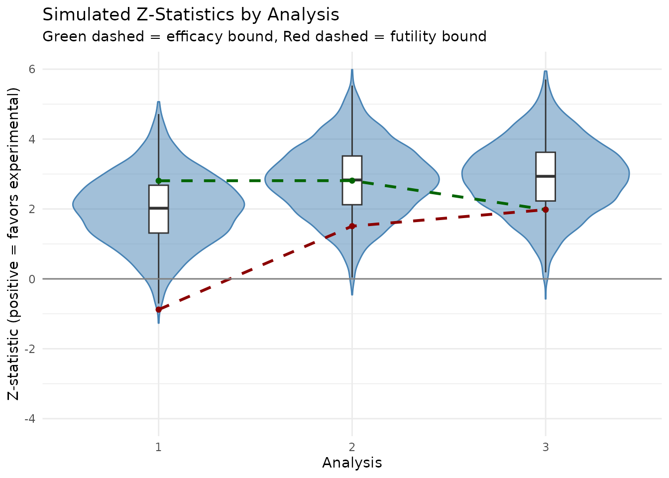

Z-statistics across analyses with group sequential boundaries

Notes

This simulation demonstrates the basic workflow for group sequential designs with negative binomial outcomes:

Sample size calculation using sample_size_nbinom() for a fixed design
Group sequential design using gsNBCalendar() to add interim analyses
Simulation using nb_sim() to generate trial data
Analysis using cut_data_by_date() and mutze_test() at each interim
Boundary checking against the group sequential bounds

The usTime = c(0.1, 0.2, 1) specification provides conservative alpha spending at early analyses, preserving most of the Type I error for later analyses when more information is available.

With only 50 simulations, the estimated power has substantial Monte Carlo error. For more precise estimates, increase n_sims to 1000 or more.