7  Comparing sample size approximation methods

This chapter compares sample size and event count approximations across packages and methods for survival trials with a proportional hazards assumption. We consider nSurv() (this package), gsDesign::nEvents(), rpact::getSampleSizeSurvival(), gsDesign2::gs_design_ahr(), and gsDesign2::gs_design_wlr().

7.1 Fixed-design sample size

We begin with a simple fixed (non-sequential) design:

  • Control median survival: 12 months (\(\lambda_C = \log 2 / 12\))
  • Hazard ratio: 0.7
  • One-sided \(\alpha = 0.025\), power \(= 90\%\) (\(\beta = 0.1\))
  • Equal randomization (ratio = 1)
  • Constant enrollment rate over 12 months
  • 24-month follow-up, no dropout
results <- data.frame(
  Source = character(), Method = character(),
  Events = numeric(), N = numeric(), stringsAsFactors = FALSE
)

# nSurv with all methods
for (m in c("LachinFoulkes", "Schoenfeld", "Freedman", "BernsteinLagakos")) {
  x <- nSurv(lambdaC = lambdaC, hr = hr_design, gamma = 10, R = 12,
    T = 36, minfup = 24, alpha = alpha, beta = beta, method = m)
  results <- rbind(results, data.frame(
    Source = "nSurv", Method = m, Events = x$d, N = x$n))
}

# gsDesign::nEvents (event count only, no N)
ne <- gsDesign::nEvents(hr = hr_design, alpha = alpha, beta = beta)
results <- rbind(results, data.frame(
  Source = "gsDesign::nEvents", Method = "Schoenfeld", Events = ne, N = NA))

# rpact
d_fixed <- getDesignGroupSequential(kMax = 1, sided = 1, alpha = alpha, beta = beta)
for (tc in c("Schoenfeld", "Freedman")) {
  ss <- getSampleSizeSurvival(d_fixed, hazardRatio = hr_design,
    lambda2 = lambdaC, accrualTime = c(0, 12), followUpTime = 24,
    typeOfComputation = tc)
  results <- rbind(results, data.frame(
    Source = "rpact", Method = tc, Events = ss$maxNumberOfEvents,
    N = ss$maxNumberOfSubjects))
}

# gsDesign2 gs_design_ahr (k=1 fixed design) with 3 info_scale options
enroll_fix <- define_enroll_rate(duration = 12, rate = 10)
fail_fix <- define_fail_rate(duration = Inf, fail_rate = lambdaC,
  hr = hr_design, dropout_rate = 0)

for (is in c("h0_h1_info", "h0_info", "h1_info")) {
  x2 <- gs_design_ahr(enroll_rate = enroll_fix, fail_rate = fail_fix,
    alpha = alpha, beta = beta, info_frac = 1, info_scale = is)
  results <- rbind(results, data.frame(
    Source = "gsDesign2 ahr", Method = is, Events = x2$analysis$event,
    N = x2$analysis$n))
}

# gsDesign2 gs_design_wlr (k=1) with 3 info_scale options
for (is in c("h0_h1_info", "h0_info", "h1_info")) {
  x_wlr <- gs_design_wlr(enroll_rate = enroll_fix, fail_rate = fail_fix,
    weight = "logrank", alpha = alpha, beta = beta,
    info_frac = 1, info_scale = is)
  results <- rbind(results, data.frame(
    Source = "gsDesign2 wlr", Method = is, Events = x_wlr$analysis$event,
    N = x_wlr$analysis$n))
}

results |>
  gt() |>
  fmt_number(columns = c("Events", "N"), decimals = 1) |>
  sub_missing(missing_text = "--") |>
  tab_header(title = "Fixed-design sample size by method and package",
    subtitle = "HR = 0.7, alpha = 0.025, beta = 0.1, ratio = 1") |>
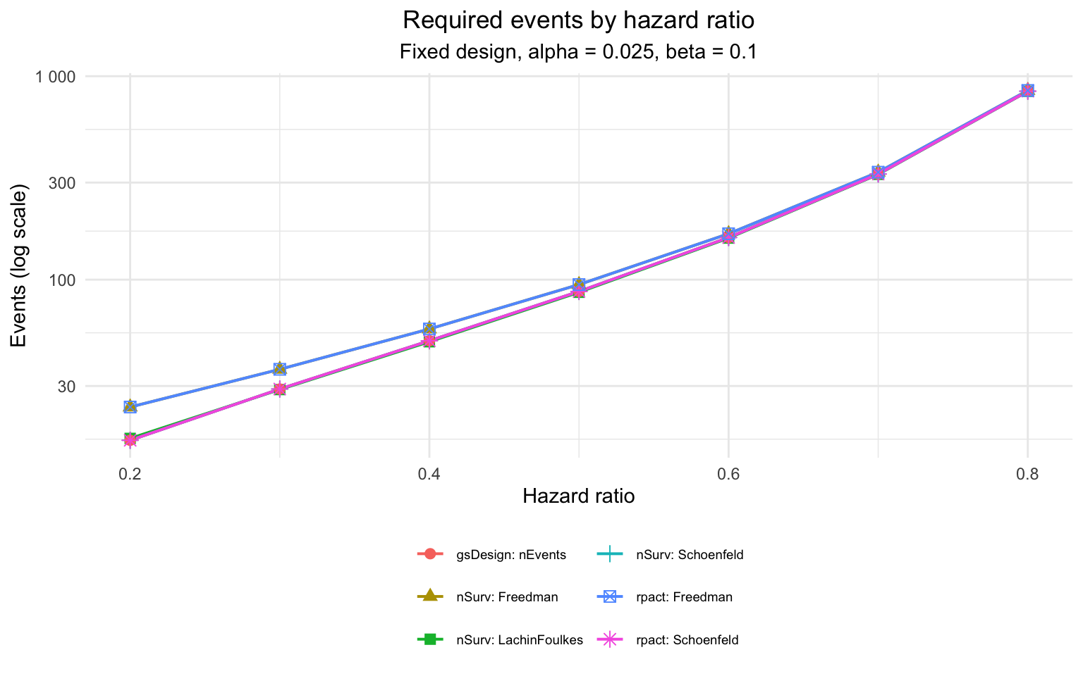
  tab_spanner(label = "Results", columns = c("Events", "N"))
Fixed-design sample size by method and package
HR = 0.7, alpha = 0.025, beta = 0.1, ratio = 1
Source Method
Results
Events N
nSurv LachinFoulkes 329.2 433.3
nSurv Schoenfeld 330.4 434.9
nSurv Freedman 337.4 444.1
nSurv BernsteinLagakos 316.5 416.5
gsDesign::nEvents Schoenfeld 330.4
rpact Schoenfeld 330.4 434.9
rpact Freedman 337.4 444.1
gsDesign2 ahr h0_h1_info 331.2 435.9
gsDesign2 ahr h0_info 332.4 437.6
gsDesign2 ahr h1_info 332.4 437.6
gsDesign2 wlr h0_h1_info 325.8 428.8
gsDesign2 wlr h0_info 330.7 435.3
gsDesign2 wlr h1_info 330.7 435.3

nSurv() Schoenfeld matches gsDesign::nEvents() and rpact Schoenfeld exactly; nSurv() Freedman matches rpact Freedman exactly. The LachinFoulkes method requires slightly fewer events because it uses both null and alternative variances. The gsDesign2::fixed_design_ahr() info_scale options produce similar but not identical results: h0_h1_info is closest to LachinFoulkes, while h0_info and h1_info use only one variance. Note that gsDesign2::fixed_design_ahr() results are based on an asymptotic approximation to the logrank test that differs slightly from the classical formulas. The gsDesign2::fixed_design_wlr() results are based on the npsurvSS R package which uses a fixed end time for enrollment, assuming enrollment is piecewise constant in that fixed time period.

7.2 Group sequential design comparison

We now compare a 3-analysis group sequential design with non-binding futility bounds (test.type = 4), Hwang-Shih-DeCani spending (\(\gamma_{\alpha} = -4\), \(\gamma_{\beta} = -2\)).

gs_results <- list()

# gsSurv designs
for (m in c("LachinFoulkes", "Schoenfeld", "Freedman")) {
  x <- gsSurv(k = 3, test.type = 4, alpha = 0.025, sided = 1, beta = 0.1,
    sfu = sfHSD, sfupar = -4, sfl = sfHSD, sflpar = -2,
    lambdaC = lambdaC, hr = hr_design, gamma = 10, R = 12,
    minfup = 24, T = 36, r = 40, method = m)
  gs_results[[paste0("gsSurv (", m, ")")]] <- list(
    events = x$n.I, N = sum(x$eNC[3, ] + x$eNE[3, ]),
    upper = x$upper$bound, lower = x$lower$bound)
}

# rpact Schoenfeld and Freedman
d_rpact <- getDesignGroupSequential(kMax = 3, typeOfDesign = "asHSD", gammaA = -4,
  sided = 1, alpha = 0.025, beta = 0.1,
  typeBetaSpending = "bsHSD", gammaB = -2,
  informationRates = c(1/3, 2/3, 1))

for (tc in c("Schoenfeld", "Freedman")) {
  ss_rp <- getSampleSizeSurvival(d_rpact, hazardRatio = hr_design,
    lambda2 = lambdaC, accrualTime = c(0, 12), followUpTime = 24,
    typeOfComputation = tc)
  gs_results[[paste0("rpact (", tc, ")")]] <- list(
    events = as.numeric(ss_rp$eventsPerStage),
    N = ss_rp$maxNumberOfSubjects,
    upper = d_rpact$criticalValues,
    lower = d_rpact$futilityBounds)
}

# gsDesign2 ahr with 3 info_scale options
enroll_gs2 <- define_enroll_rate(duration = 12, rate = 10)
fail_gs2 <- define_fail_rate(duration = Inf, fail_rate = lambdaC,
  hr = hr_design, dropout_rate = 0)

for (is in c("h0_h1_info", "h0_info", "h1_info")) {
  x2 <- gs_design_ahr(enroll_rate = enroll_gs2, fail_rate = fail_gs2,
    alpha = 0.025, beta = 0.1, info_frac = c(1/3, 2/3, 1),
    info_scale = is,
    upper = gs_spending_bound, upar = list(sf = sfHSD, param = -4, total_spend = 0.025),
    lower = gs_spending_bound, lpar = list(sf = sfHSD, param = -2, total_spend = 0.1),
    binding = FALSE)
  gs_results[[paste0("gsDesign2 ahr (", is, ")")]] <- list(
    events = x2$analysis$event,
    N = max(x2$analysis$n),
    upper = x2$bound$z[x2$bound$bound == "upper"],
    lower = x2$bound$z[x2$bound$bound == "lower"])
}

# gsDesign2 wlr logrank with 3 info_scale options
for (is in c("h0_h1_info", "h0_info", "h1_info")) {
  x_wlr <- gs_design_wlr(enroll_rate = enroll_gs2, fail_rate = fail_gs2,
    weight = "logrank", alpha = 0.025, beta = 0.1,
    info_frac = c(1/3, 2/3, 1), info_scale = is,
    upper = gs_spending_bound, upar = list(sf = sfHSD, param = -4, total_spend = 0.025),
    lower = gs_spending_bound, lpar = list(sf = sfHSD, param = -2, total_spend = 0.1),
    binding = FALSE)
  gs_results[[paste0("gsDesign2 wlr (", is, ")")]] <- list(
    events = x_wlr$analysis$event,
    N = max(x_wlr$analysis$n),
    upper = x_wlr$bound$z[x_wlr$bound$bound == "upper"],
    lower = x_wlr$bound$z[x_wlr$bound$bound == "lower"])
}

# Build comparison table
gs_tab <- do.call(rbind, lapply(names(gs_results), function(nm) {
  r <- gs_results[[nm]]
  data.frame(
    Source = nm,
    Final_Events = round(max(r$events), 1),
    N = round(r$N, 1),
    Upper_1 = round(r$upper[1], 4),
    Upper_2 = round(r$upper[2], 4),
    Upper_3 = round(r$upper[3], 4),
    Lower_1 = round(r$lower[1], 4),
    Lower_2 = round(r$lower[2], 4),
    stringsAsFactors = FALSE)
}))

gs_tab |>
  gt() |>
  tab_header(title = "Group sequential design comparison",
    subtitle = "k = 3, HSD spending, HR = 0.7, alpha = 0.025, beta = 0.1") |>
  tab_spanner(label = "Efficacy bounds (Z)", columns = starts_with("Upper")) |>
  tab_spanner(label = "Futility bounds (Z)", columns = starts_with("Lower")) |>
  cols_label(
    Final_Events = "Final events",
    Upper_1 = "IA1", Upper_2 = "IA2", Upper_3 = "FA",
    Lower_1 = "IA1", Lower_2 = "IA2")
Group sequential design comparison
k = 3, HSD spending, HR = 0.7, alpha = 0.025, beta = 0.1
Source Final events N
Efficacy bounds (Z)
Futility bounds (Z)
IA1 IA2 FA IA1 IA2
gsSurv (LachinFoulkes) 352.2 463.6 3.0107 2.5465 1.9992 -0.2388 0.9410
gsSurv (Schoenfeld) 353.5 465.2 3.0107 2.5465 1.9992 -0.2388 0.9410
gsSurv (Freedman) 361.0 475.1 3.0107 2.5465 1.9992 -0.2388 0.9410
rpact (Schoenfeld) 353.5 465.3 3.0107 2.5465 1.9992 -0.2387 0.9411
rpact (Freedman) 361.0 475.2 3.0107 2.5465 1.9992 -0.2387 0.9411
gsDesign2 ahr (h0_h1_info) 345.0 454.1 3.0107 2.5465 1.9992 -0.2904 0.8817
gsDesign2 ahr (h0_info) 355.7 468.2 3.0107 2.5465 1.9992 -0.2387 0.9411
gsDesign2 ahr (h1_info) 355.4 467.9 3.0190 2.5549 1.9986 -0.2621 0.9220
gsDesign2 wlr (h0_h1_info) 351.0 462.0 3.0107 2.5465 1.9992 -0.2412 0.9379
gsDesign2 wlr (h0_info) 354.1 466.1 3.0107 2.5465 1.9992 -0.2605 0.9226
gsDesign2 wlr (h1_info) 354.1 466.1 3.0107 2.5465 1.9992 -0.2607 0.9222

Note that sample sizes (N) depend on the enrollment assumptions and how each package scales enrollment to achieve the required events. The event counts and Z-bounds are the primary quantities for comparison. The Schoenfeld-based methods (gsSurv, rpact) essentially identical event counts, sample size and bounds. The gsDesign2 results with h0_h1_info are closest to LachinFoulkes. Bounds are nearly identical across packages for matching spending functions.

7.3 Event counts across hazard ratios

We compare required events across HR = 0.2 to 0.8 to see how methods diverge, especially at extreme HRs where asymptotic approximations are tested.

hr_grid <- seq(0.2, 0.8, by = 0.1)

hr_rows <- list()
for (h in hr_grid) {
  for (m in c("LachinFoulkes", "Schoenfeld", "Freedman")) {
    x <- nSurv(lambdaC = lambdaC, hr = h, gamma = 10, R = 12,
      T = 36, minfup = 24, alpha = alpha, beta = beta, method = m)
    hr_rows <- c(hr_rows, list(data.frame(
      HR = h, Source = "nSurv", Method = m, Events = x$d)))
  }

  ne <- gsDesign::nEvents(hr = h, alpha = alpha, beta = beta)
  hr_rows <- c(hr_rows, list(data.frame(
    HR = h, Source = "gsDesign", Method = "nEvents", Events = ne)))

  for (tc in c("Schoenfeld", "Freedman")) {
    ss <- getSampleSizeSurvival(d_fixed, hazardRatio = h,
      lambda2 = lambdaC, accrualTime = c(0, 12), followUpTime = 24,
      typeOfComputation = tc)
    hr_rows <- c(hr_rows, list(data.frame(
      HR = h, Source = "rpact", Method = tc, Events = ss$maxNumberOfEvents)))
  }
}
hr_results <- do.call(rbind, hr_rows)

# Table with column spanners
hr_results$label <- paste0(hr_results$Source, ": ", hr_results$Method)
hr_wide <- reshape(hr_results[, c("HR", "label", "Events")],
  idvar = "HR", timevar = "label", direction = "wide")
names(hr_wide) <- sub("Events\\.", "", names(hr_wide))

lf_cols <- grep("LachinFoulkes", names(hr_wide), value = TRUE)
sch_cols <- grep("Schoenfeld|nEvents", names(hr_wide), value = TRUE)
fre_cols <- grep("Freedman", names(hr_wide), value = TRUE)

hr_wide |>
  gt() |>
  fmt_number(columns = -1, decimals = 1) |>
  tab_header(title = "Required events by hazard ratio, method, and package",
    subtitle = "Fixed design, alpha = 0.025, beta = 0.1, ratio = 1") |>
  tab_spanner(label = "Schoenfeld", columns = all_of(sch_cols)) |>
  tab_spanner(label = "Freedman", columns = all_of(fre_cols))
Required events by hazard ratio, method, and package
Fixed design, alpha = 0.025, beta = 0.1, ratio = 1
HR nSurv: LachinFoulkes
Schoenfeld
Freedman
nSurv: Schoenfeld gsDesign: nEvents rpact: Schoenfeld nSurv: Freedman rpact: Freedman
0.2 16.6 16.2 16.2 16.2 23.6 23.6
0.3 28.8 29.0 29.0 29.0 36.2 36.2
0.4 49.5 50.1 50.1 50.1 57.2 57.2
0.5 86.6 87.5 87.5 87.5 94.6 94.6
0.6 160.0 161.1 161.1 161.1 168.1 168.1
0.7 329.2 330.4 330.4 330.4 337.4 337.4
0.8 842.8 844.1 844.1 844.1 851.1 851.1
# Consolidated table: one column per method (since packages agree)
# Add gsDesign2 ahr results for the same HR grid
enroll_hr <- define_enroll_rate(duration = 12, rate = 10)
hr_consol <- data.frame(HR = hr_grid)
hr_consol$LachinFoulkes <- sapply(hr_grid, function(h)
  nSurv(lambdaC = lambdaC, hr = h, gamma = 10, R = 12, T = 36, minfup = 24,
    alpha = alpha, beta = beta, method = "LachinFoulkes")$d)
hr_consol$Schoenfeld <- sapply(hr_grid, function(h)
  gsDesign::nEvents(hr = h, alpha = alpha, beta = beta))
hr_consol$Freedman <- sapply(hr_grid, function(h)
  nSurv(lambdaC = lambdaC, hr = h, gamma = 10, R = 12, T = 36, minfup = 24,
    alpha = alpha, beta = beta, method = "Freedman")$d)

for (is in c("h0_h1_info", "h0_info", "h1_info")) {
  hr_consol[[paste0("ahr_", is)]] <- sapply(hr_grid, function(h) {
    fail_h <- define_fail_rate(duration = Inf, fail_rate = lambdaC,
      hr = h, dropout_rate = 0)
    gs_design_ahr(enroll_rate = enroll_hr, fail_rate = fail_h,
      alpha = alpha, beta = beta, info_frac = 1,
      info_scale = is)$analysis$event
  })
}

hr_consol |>
  gt() |>
  fmt_number(columns = -1, decimals = 1) |>
  tab_header(title = "Required events by method (consolidated)",
    subtitle = "One column per method; packages producing identical results are merged") |>
  cols_label(
    ahr_h0_h1_info = "h0_h1_info",
    ahr_h0_info = "h0_info",
    ahr_h1_info = "h1_info") |>
  tab_spanner(label = "Classical methods", columns = c("LachinFoulkes", "Schoenfeld", "Freedman")) |>
  tab_spanner(label = "gsDesign2 ahr info_scale", columns = starts_with("ahr_"))
Required events by method (consolidated)
One column per method; packages producing identical results are merged
HR
Classical methods
gsDesign2 ahr info_scale
LachinFoulkes Schoenfeld Freedman h0_h1_info h0_info h1_info
0.2 16.6 16.2 23.6 18.0 20.9 20.9
0.3 28.8 29.0 36.2 30.5 32.8 32.8
0.4 49.5 50.1 57.2 51.3 53.2 53.2
0.5 86.6 87.5 94.6 88.5 90.2 90.2
0.6 160.0 161.1 168.1 162.0 163.4 163.4
0.7 329.2 330.4 337.4 331.2 332.4 332.4
0.8 842.8 844.1 851.1 844.8 845.9 845.9
# Plot
print(
  ggplot(hr_results, aes(x = HR, y = Events, color = label, shape = label)) +
    geom_line(linewidth = 0.7) +
    geom_point(size = 2.5) +
    scale_y_log10(labels = scales::label_number()) +
    labs(title = "Required events by hazard ratio",
      subtitle = "Fixed design, alpha = 0.025, beta = 0.1",
      x = "Hazard ratio", y = "Events (log scale)", color = NULL, shape = NULL) +
    theme_minimal() +
    theme(
      legend.position = "bottom",
      plot.title = element_text(hjust = 0.5),
      plot.subtitle = element_text(hjust = 0.5),
      legend.text = element_text(size = 7)) +
    guides(color = guide_legend(ncol = 2), shape = guide_legend(ncol = 2))
)

At moderate HRs (0.5–0.8), the methods agree closely. At extreme HRs (0.2–0.3), the methods diverge substantially:

  • Schoenfeld requires the fewest events but relies on a local-alternative approximation that breaks down for large effects.
  • Freedman requires more events, using a non-log parameterization (\(\delta = (\text{hr} - 1) / (\text{hr} + 1/\text{ratio})\)) that is more conservative for extreme HRs.
  • LachinFoulkes falls between the two, using both null and alternative variances for a tighter estimate.

Note that nSurv() Schoenfeld, gsDesign::nEvents(), and rpact Schoenfeld lines overlap exactly in the plot. Similarly, nSurv() Freedman and rpact Freedman overlap. The only visually distinct line is Freedman, which diverges at low HRs.

7.4 Type I error at extreme hazard ratios

With HR = 0.2, the Schoenfeld method requires only 17 events while Freedman requires 24. With so few events, asymptotic approximations may not control Type I error at the nominal level. We use simtrial::sim_fixed_n() to simulate 100,000 trials under the null hypothesis (HR = 1) for each method’s event count.

library(simtrial)
library(future)
plan(multisession, workers = parallelly::availableCores())

# Collect event counts from all methods including gsDesign2
all_methods <- data.frame(
  Label = character(), Events = integer(), N = integer(),
  stringsAsFactors = FALSE
)

for (m in c("LachinFoulkes", "Schoenfeld", "Freedman", "BernsteinLagakos")) {
  x <- nSurv(lambdaC = lambdaC, hr = 0.2, gamma = 10, R = 12,
    T = 36, minfup = 24, alpha = alpha, beta = beta, method = m)
  all_methods <- rbind(all_methods, data.frame(
    Label = paste0("nSurv: ", m), Events = ceiling(x$d), N = ceiling(x$n)))
}

enroll_02 <- define_enroll_rate(duration = 12, rate = 10)
fail_02 <- define_fail_rate(duration = Inf, fail_rate = lambdaC, hr = 0.2, dropout_rate = 0)

for (fn in c("gs_design_ahr", "gs_design_wlr")) {
  short <- if (fn == "gs_design_ahr") "ahr" else "wlr"
  for (is in c("h0_h1_info", "h0_info", "h1_info")) {
    args <- list(enroll_rate = enroll_02, fail_rate = fail_02,
      alpha = alpha, beta = beta, info_frac = 1, info_scale = is)
    if (fn == "gs_design_wlr") args$weight <- "logrank"
    x2 <- do.call(fn, args)
    all_methods <- rbind(all_methods, data.frame(
      Label = paste0("gsDesign2 ", short, ": ", is),
      Events = ceiling(x2$analysis$event), N = ceiling(x2$analysis$n)))
  }
}

# Deduplicate: only simulate once per unique event count
unique_events <- unique(all_methods$Events)
n_sim <- 100000

sim_cache <- list()
for (ev in unique_events) {
  set.seed(20260123)
  sim <- sim_fixed_n(
    n_sim = n_sim,
    sample_size = 400,
    target_event = ev,
    enroll_rate = data.frame(duration = 12, rate = 400 / 12),
    fail_rate = data.frame(
      stratum = "All", duration = Inf,
      fail_rate = lambdaC, hr = 1, dropout_rate = 0
    ),
    total_duration = 100,
    timing_type = 2,
    rho_gamma = data.frame(rho = 0, gamma = 0, rho_gamma = "0 0")
  )
  sim_cache[[as.character(ev)]] <- sum(sim$z >= qnorm(1 - alpha))
}

sim_results <- data.frame(
  Label = all_methods$Label,
  Events = all_methods$Events,
  N = all_methods$N,
  Rejections = sapply(all_methods$Events, function(ev) sim_cache[[as.character(ev)]]),
  Alpha = sapply(all_methods$Events, function(ev) sim_cache[[as.character(ev)]]) / n_sim
)

plan(sequential)
sim_results$Nominal <- alpha
sim_results$Ratio <- sim_results$Alpha / alpha

sim_results |>
  gt() |>
  fmt_number(columns = c("Alpha", "Nominal"), decimals = 4) |>
  fmt_number(columns = "Ratio", decimals = 2) |>
  tab_header(
    title = "Simulated Type I error by method (HR = 0.2 event counts)",
    subtitle = sprintf("%s trials under H0 (HR = 1), nominal alpha = %.3f",
      format(n_sim, big.mark = ","), alpha)
  ) |>
  cols_label(
    Label = "Method", Events = "Target events",
    Rejections = "Rejections", Alpha = "Simulated alpha",
    Nominal = "Nominal alpha", Ratio = "Inflation ratio")
Simulated Type I error by method (HR = 0.2 event counts)
1e+05 trials under H0 (HR = 1), nominal alpha = 0.025
Method Target events N Rejections Simulated alpha Nominal alpha Inflation ratio
nSurv: LachinFoulkes 17 30 1882 0.0188 0.0250 0.75
nSurv: Schoenfeld 17 30 1882 0.0188 0.0250 0.75
nSurv: Freedman 24 43 2203 0.0220 0.0250 0.88
nSurv: BernsteinLagakos 15 27 2410 0.0241 0.0250 0.96
gsDesign2 ahr: h0_h1_info 19 33 2197 0.0220 0.0250 0.88
gsDesign2 ahr: h0_info 21 38 2685 0.0268 0.0250 1.07
gsDesign2 ahr: h1_info 21 38 2685 0.0268 0.0250 1.07
gsDesign2 wlr: h0_h1_info 16 28 2838 0.0284 0.0250 1.14
gsDesign2 wlr: h0_info 18 33 3074 0.0307 0.0250 1.23
gsDesign2 wlr: h1_info 18 33 3074 0.0307 0.0250 1.23

Each unique event count is simulated once with the same seed, so methods producing identical event counts share the same simulation result. We note that for small event counts, the asymptotic approximations of Type I error and power may be less accurate than for larger event counts. The discrete nature of the possible outcomes is the reason for this. Exact methods, including just doing a large simulation, may be preferred. We see in the table that Type I error is well-controlled for some event counts, but not for others.

7.5 Simulated power at HR = 0.2

We also verify that each method achieves approximately 90% power at its design HR of 0.2 by simulating 1,000 trials under H1. Each method uses the same seed for comparability; methods with identical event counts and sample sizes share a single simulation.

library(simtrial)
library(future)
plan(multisession, workers = parallelly::availableCores())

n_pwr <- 1000

# Unique (events, N) combinations
pwr_keys <- unique(all_methods[, c("Events", "N")])
pwr_cache <- list()

for (j in seq_len(nrow(pwr_keys))) {
  ev <- pwr_keys$Events[j]
  n_subj <- pwr_keys$N[j]
  key <- paste(ev, n_subj, sep = "_")
  set.seed(20260124)
  sim <- sim_fixed_n(
    n_sim = n_pwr,
    sample_size = n_subj,
    target_event = ev,
    enroll_rate = data.frame(duration = 12, rate = n_subj / 12),
    fail_rate = data.frame(
      stratum = "All", duration = Inf,
      fail_rate = lambdaC, hr = 0.2, dropout_rate = 0
    ),
    total_duration = 100,
    timing_type = 2,
    rho_gamma = data.frame(rho = 0, gamma = 0, rho_gamma = "0 0")
  )
  pwr_cache[[key]] <- sum(sim$z >= qnorm(1 - alpha))
}

pwr_sim <- data.frame(
  Label = all_methods$Label,
  Events = all_methods$Events,
  N = all_methods$N,
  Rejections = sapply(seq_len(nrow(all_methods)), function(i) {
    pwr_cache[[paste(all_methods$Events[i], all_methods$N[i], sep = "_")]]
  }),
  stringsAsFactors = FALSE
)
pwr_sim$Power <- pwr_sim$Rejections / n_pwr

plan(sequential)
pwr_sim$Target <- 1 - beta

pwr_sim |>
  gt() |>
  fmt_number(columns = c("Power", "Target"), decimals = 3) |>
  tab_header(
    title = "Simulated power by method (HR = 0.2)",
    subtitle = sprintf("%s trials under H1 (HR = 0.2), target power = %.0f%%",
      format(n_pwr, big.mark = ","), (1 - beta) * 100)
  ) |>
  cols_label(
    Label = "Method", Events = "Target events", N = "Sample size",
    Rejections = "Rejections", Power = "Simulated power",
    Target = "Target power")
Simulated power by method (HR = 0.2)
1,000 trials under H1 (HR = 0.2), target power = 90%
Method Target events Sample size Rejections Simulated power Target power
nSurv: LachinFoulkes 17 30 866 0.866 0.900
nSurv: Schoenfeld 17 30 866 0.866 0.900
nSurv: Freedman 24 43 961 0.961 0.900
nSurv: BernsteinLagakos 15 27 830 0.830 0.900
gsDesign2 ahr: h0_h1_info 19 33 899 0.899 0.900
gsDesign2 ahr: h0_info 21 38 935 0.935 0.900
gsDesign2 ahr: h1_info 21 38 935 0.935 0.900
gsDesign2 wlr: h0_h1_info 16 28 863 0.863 0.900
gsDesign2 wlr: h0_info 18 33 886 0.886 0.900
gsDesign2 wlr: h1_info 18 33 886 0.886 0.900

All methods achieve approximately 90% simulated power at HR = 0.2, confirming that the different event counts each calibrate correctly for the design HR despite the small sample sizes.

7.6 Design for rare events

For background on using a time-to-event approximation to construct an exact-binomial rare-event design, see the gsDesign vaccine efficacy vignette “Vaccine efficacy trial design”, which builds on the exact binomial framework of Chan and Bohidar (Chan and Bohidar 1998), the group sequential theory of Jennison and Turnbull (Jennison and Turnbull 2000), and the survival approximation of Lachin and Foulkes (Lachin and Foulkes 1986). While rare-event applications are often framed as non-inferiority or vaccine-efficacy problems, the same ideas help interpret small-event-count superiority designs such as the ones studied here.

We now make events rarer than in the previous section:

  • Control hazard rate: lambdaC = 0.04 per year
  • Randomization ratio: ratio = 2
  • Alternative hazard ratio: hr = 0.2
  • Enrollment duration: 1 year
  • Total study duration: 2 years
  • No dropout

The table below compares asymptotic event-count methods and adds a conservative exact-binomial comparator using nBinomial1Sample(). Following the rare-event/binomial logic in the vaccine-efficacy vignette, we define a “success” as an event in the control arm. Under hr0 = 1, the null and alternative probabilities that a given event is in the control arm are p0 = 1 / (1 + ratio) and p1 = 1 / (1 + ratio * hr), respectively.

rare_lambdaC <- 0.04
rare_ratio <- 2
rare_hr <- 0.2
rare_R <- 1
rare_T <- 2
rare_minfup <- 1

rare_rows <- list()

for (m in c("LachinFoulkes", "Schoenfeld", "Freedman", "BernsteinLagakos")) {
  x <- nSurv(
    lambdaC = rare_lambdaC, hr = rare_hr, gamma = 10, R = rare_R,
    T = rare_T, minfup = rare_minfup, ratio = rare_ratio,
    alpha = alpha, beta = beta, method = m
  )
  rare_rows <- c(rare_rows, list(data.frame(
    Label = paste0("nSurv: ", m),
    Events = ceiling(x$d),
    N = ceiling(x$n),
    stringsAsFactors = FALSE
  )))
}

rare_p0 <- 1 / (1 + rare_ratio)
rare_p1 <- 1 / (1 + rare_ratio * rare_hr)
nb1 <- nBinomial1Sample(
  p0 = rare_p0, p1 = rare_p1,
  alpha = alpha, beta = beta,
  n = 1:200, outtype = 2, conservative = TRUE
)
rare_rows <- c(rare_rows, list(data.frame(
  Label = "Exact binomial: nBinomial1Sample(conservative = TRUE)",
  Events = nb1$n,
  N = NA_real_,
  stringsAsFactors = FALSE
)))

rare_tab <- do.call(rbind, rare_rows)
rare_tab$Critical <- ifelse(
  grepl("^Exact binomial", rare_tab$Label),
  nb1$b,
  qbinom(1 - alpha, rare_tab$Events, rare_p0) + 1
)
rare_tab$ExactAlpha <- ifelse(
  grepl("^Exact binomial", rare_tab$Label),
  nb1$alphaR,
  pbinom(rare_tab$Critical - 1, rare_tab$Events, rare_p0, lower.tail = FALSE)
)
rare_tab$ExactPower <- ifelse(
  grepl("^Exact binomial", rare_tab$Label),
  nb1$Power,
  pbinom(rare_tab$Critical - 1, rare_tab$Events, rare_p1, lower.tail = FALSE)
)

rare_tab |>
  gt() |>
  sub_missing(missing_text = "--") |>
  fmt_number(columns = c("ExactAlpha", "ExactPower"), decimals = 4) |>
  tab_header(
    title = "Rare-event design: asymptotic sample size and exact-binomial operating characteristics",
    subtitle = "lambdaC = 0.04/year, ratio = 2 (experimental:control), hr = 0.2, 1-year enrollment, 2-year trial"
  ) |>
  cols_label(
    Label = "Method", Events = "Target events", N = "Sample size",
    Critical = "Min control events to reject",
    ExactAlpha = "Exact alpha", ExactPower = "Exact power"
  )
Rare-event design: asymptotic sample size and exact-binomial operating characteristics
lambdaC = 0.04/year, ratio = 2 (experimental:control), hr = 0.2, 1-year enrollment, 2-year trial
Method Target events Sample size Min control events to reject Exact alpha Exact power
nSurv: LachinFoulkes 19 685 11 0.0241 0.9362
nSurv: Schoenfeld 19 668 11 0.0241 0.9362
nSurv: Freedman 17 589 11 0.0080 0.8136
nSurv: BernsteinLagakos 13 455 9 0.0088 0.6966
Exact binomial: nBinomial1Sample(conservative = TRUE) 19 11 0.0241 0.9362

With a 2:1 (experimental:control) randomization ratio, each event is assigned to control with probability \(p_0 = 1/3\) under \(H_0\) and \(p_1 = 5/7\) under \(H_1\) (\(\text{hr} = 0.2\)). The exact-binomial test rejects when the number of control-arm events reaches or exceeds the critical value shown. Methods with smaller event counts can look optimistic in this setting because the binomial discreteness is no longer negligible. The nBinomial1Sample(conservative = TRUE) row provides a conservative benchmark that ensures power is at least 90% for all event counts at or above the selected value.

library(simtrial)
library(future)
plan(multisession, workers = parallelly::availableCores())

rare_sim_tab <- subset(rare_tab, !is.na(N))
rare_keys <- unique(rare_sim_tab[, c("Events", "N")])
n_rare_alpha <- 5000
n_rare_power <- 1000
rare_alpha_cache <- list()
rare_power_cache <- list()

for (j in seq_len(nrow(rare_keys))) {
  ev <- rare_keys$Events[j]
  n_subj <- rare_keys$N[j]
  key <- paste(ev, n_subj, sep = "_")

  set.seed(20260125)
  sim0 <- sim_fixed_n(
    n_sim = n_rare_alpha,
    sample_size = n_subj,
    target_event = ev,
    enroll_rate = data.frame(duration = rare_R, rate = n_subj / rare_R),
    fail_rate = data.frame(
      stratum = "All", duration = Inf,
      fail_rate = rare_lambdaC, hr = 1, dropout_rate = 0
    ),
    total_duration = 10,
    timing_type = 2,
    rho_gamma = data.frame(rho = 0, gamma = 0, rho_gamma = "0 0")
  )
  rare_alpha_cache[[key]] <- sum(sim0$z >= qnorm(1 - alpha))

  set.seed(20260126)
  sim1 <- sim_fixed_n(
    n_sim = n_rare_power,
    sample_size = n_subj,
    target_event = ev,
    enroll_rate = data.frame(duration = rare_R, rate = n_subj / rare_R),
    fail_rate = data.frame(
      stratum = "All", duration = Inf,
      fail_rate = rare_lambdaC, hr = rare_hr, dropout_rate = 0
    ),
    total_duration = 10,
    timing_type = 2,
    rho_gamma = data.frame(rho = 0, gamma = 0, rho_gamma = "0 0")
  )
  rare_power_cache[[key]] <- sum(sim1$z >= qnorm(1 - alpha))
}

rare_tab$SimAlpha <- sapply(seq_len(nrow(rare_tab)), function(i) {
  if (is.na(rare_tab$N[i])) return(NA_real_)
  rare_alpha_cache[[paste(rare_tab$Events[i], rare_tab$N[i], sep = "_")]] / n_rare_alpha
})
rare_tab$SimPower <- sapply(seq_len(nrow(rare_tab)), function(i) {
  if (is.na(rare_tab$N[i])) return(NA_real_)
  rare_power_cache[[paste(rare_tab$Events[i], rare_tab$N[i], sep = "_")]] / n_rare_power
})

plan(sequential)
rare_tab |>
  gt() |>
  sub_missing(missing_text = "--") |>
  fmt_number(columns = c("ExactAlpha", "ExactPower", "SimAlpha", "SimPower"), decimals = 4) |>
  tab_header(
    title = "Rare-event design: exact-binomial vs survival-trial simulation",
    subtitle = sprintf(
      "ratio = 2 (experimental:control); Type I error from %s H0 trials and power from %s H1 trials",
      format(n_rare_alpha, big.mark = ","), format(n_rare_power, big.mark = ",")
    )
  ) |>
  cols_label(
    Label = "Method", Events = "Target events", N = "Sample size",
    ExactAlpha = "Exact alpha", ExactPower = "Exact power",
    SimAlpha = "Simulated alpha", SimPower = "Simulated power"
  )
Rare-event design: exact-binomial vs survival-trial simulation
ratio = 2 (experimental:control); Type I error from 5,000 H0 trials and power from 1,000 H1 trials
Method Target events Sample size Critical Exact alpha Exact power Simulated alpha Simulated power
nSurv: LachinFoulkes 19 685 11 0.0241 0.9362 0.0286 0.9120
nSurv: Schoenfeld 19 668 11 0.0241 0.9362 0.0282 0.9190
nSurv: Freedman 17 589 11 0.0080 0.8136 0.0202 0.8580
nSurv: BernsteinLagakos 13 455 9 0.0088 0.6966 0.0320 0.7900
Exact binomial: nBinomial1Sample(conservative = TRUE) 19 11 0.0241 0.9362

This rare-event section gives a practical check on how well the event-count approximations behave when the event total is very small. The exact-binomial row is a conservative benchmark based only on the discrete event-count problem. The simtrial results show how closely the underlying survival-trial designs track that benchmark once enrollment and time-to-event variation are introduced.

7.7 Key takeaways

  • nSurv() Schoenfeld matches gsDesign::nEvents() and rpact Schoenfeld exactly; nSurv() Freedman matches rpact Freedman exactly.
  • LachinFoulkes typically requires slightly fewer events than Schoenfeld because it uses both null and alternative variances. However, in the just noted rare events scenario we saw a slightly larger sample size with LachinFoulkes but the same event requirement as the Schoenfeld method. This is likely due to the LachinFoulkes method accounting for slower event accumulation under the alternate hypothesis.
  • gsDesign2 info_scale options correspond to different variance assumptions: h0_h1_info is analogous to LachinFoulkes (both variances), h0_info to Schoenfeld (null variance only), and h1_info to BernsteinLagakos (alternative variance). The gsDesign2 results are based on the asymptotic framework of Zhao, Zhang, and Anderson (2024), which uses numerical integration of the expected information under piecewise enrollment and failure models. This approach supports non-proportional hazards as well as proportional hazards and differs slightly from the classical closed-form formulas used by nSurv(), gsDesign::nEvents(), and rpact.
  • For proportional hazards with the logrank test, gs_design_wlr() and gs_design_ahr() give similar results, with small differences due to their distinct approximation approaches.
  • At extreme HRs (HR = 0.2), methods diverge substantially in required events. Regardless of method, the discrete nature of results when event counts are small are worth considering. This can be evaluated with the exact methods or large simulations.
  • For most practical designs (HR = 0.5–0.8), all methods agree closely and the choice of method has minimal impact.