4.0: Spending function overview

Spending functions are used to set boundaries for group sequential designs. Using the spending function approach to design offers a natural way to provide interim testing boundaries when unplanned interim analyses are added or when the timing of an interim analysis changes. Many standard and investigational spending functions are provided in the gsDesign package. These offer a great deal of flexibility in setting up stopping boundaries for a design.

Arguments

alpha: Real value \(> 0\) and no more than 1. Defaults in calls to gsDesign() are alpha=0.025 for one-sided Type I error specification and alpha=0.1 for Type II error specification. However, this could be set to 1 if, for descriptive purposes, you wish to see the proportion of spending as a function of the proportion of sample size/information.
t: A vector of points with increasing values from 0 to 1, inclusive. Values of the proportion of sample size/information for which the spending function will be computed.
param: A single real value or a vector of real values specifying the spending function parameter(s); this must be appropriately matched to the spending function specified.
object: A spendfn object to be summarized.
...: Not currently used.

Value

spendingFunction and spending functions in general produce an object of type spendfn.

name: A character string with the name of the spending function.
param: any parameters used for the spending function.
parname: a character string or strings with the name(s) of the parameter(s) in param.
sf: the spending function specified.
spend: a vector of cumulative spending values corresponding to the input values in t.
bound: this is null when returned from the spending function, but is set in gsDesign() if the spending function is called from there. Contains z-values for bounds of a design.
prob: this is null when returned from the spending function, but is set in gsDesign() if the spending function is called from there. Contains probabilities of boundary crossing at i-th analysis for j-th theta value input to gsDesign() in prob[i,j].

Details

The summary() function for spendfn objects provides a brief textual summary of a spending function or boundary used for a design.

Spending functions have three arguments as noted above and return an object of type spendfn. Normally a spending function will be passed to gsDesign() in the parameter sfu for the upper bound and sfl for the lower bound to specify a spending function family for a design. In this case, the user does not need to know the calling sequence - only how to specify the parameter(s) for the spending function. The calling sequence is useful when the user wishes to plot a spending function as demonstrated below in examples. In addition to using supplied spending functions, a user can write code for a spending function. See examples.

Note

The gsDesign technical manual is available at https://keaven.github.io/gsd-tech-manual/.

References

Jennison C and Turnbull BW (2000), Group Sequential Methods with Applications to Clinical Trials. Boca Raton: Chapman and Hall.

Author

Keaven Anderson keaven_anderson@merck.com

Examples

library(ggplot2)
# Example 1: simple example showing what mose users need to know

# design a 4-analysis trial using a Hwang-Shih-DeCani spending function 
# for both lower and upper bounds 
x <- gsDesign(k=4, sfu=sfHSD, sfupar=-2, sfl=sfHSD, sflpar=1)

# print the design
x
#> Asymmetric two-sided group sequential design with
#> 90 % power and 2.5 % Type I Error.
#> Upper bound spending computations assume
#> trial continues if lower bound is crossed.
#> 
#>            Sample
#>             Size   ----Lower bounds----  ----Upper bounds-----
#>   Analysis Ratio*  Z   Nominal p Spend+  Z   Nominal p Spend++
#>          1  0.324 0.03    0.5136 0.0350 2.80    0.0025  0.0025
#>          2  0.649 0.88    0.8096 0.0273 2.58    0.0049  0.0042
#>          3  0.973 1.51    0.9349 0.0212 2.34    0.0096  0.0069
#>          4  1.297 2.09    0.9817 0.0165 2.09    0.0183  0.0114
#>      Total                       0.1000                 0.0250 
#> + lower bound beta spending (under H1):
#>  Hwang-Shih-DeCani spending function with gamma = 1.
#> ++ alpha spending:
#>  Hwang-Shih-DeCani spending function with gamma = -2.
#> * Sample size ratio compared to fixed design with no interim
#> 
#> Boundary crossing probabilities and expected sample size
#> assume any cross stops the trial
#> 
#> Upper boundary (power or Type I Error)
#>           Analysis
#>    Theta      1      2      3      4  Total   E{N}
#>   0.0000 0.0025 0.0042 0.0065 0.0072 0.0203 0.5477
#>   3.2415 0.1695 0.3553 0.2774 0.0978 0.9000 0.7533
#> 
#> Lower boundary (futility or Type II Error)
#>           Analysis
#>    Theta      1      2      3      4  Total
#>   0.0000 0.5136 0.3156 0.1169 0.0336 0.9797
#>   3.2415 0.0350 0.0273 0.0212 0.0165 0.1000
# summarize the spending functions
summary(x$upper)
#> [1] "Hwang-Shih-DeCani spending function with gamma = -2"
summary(x$lower)
#> [1] "Hwang-Shih-DeCani spending function with gamma = 1"

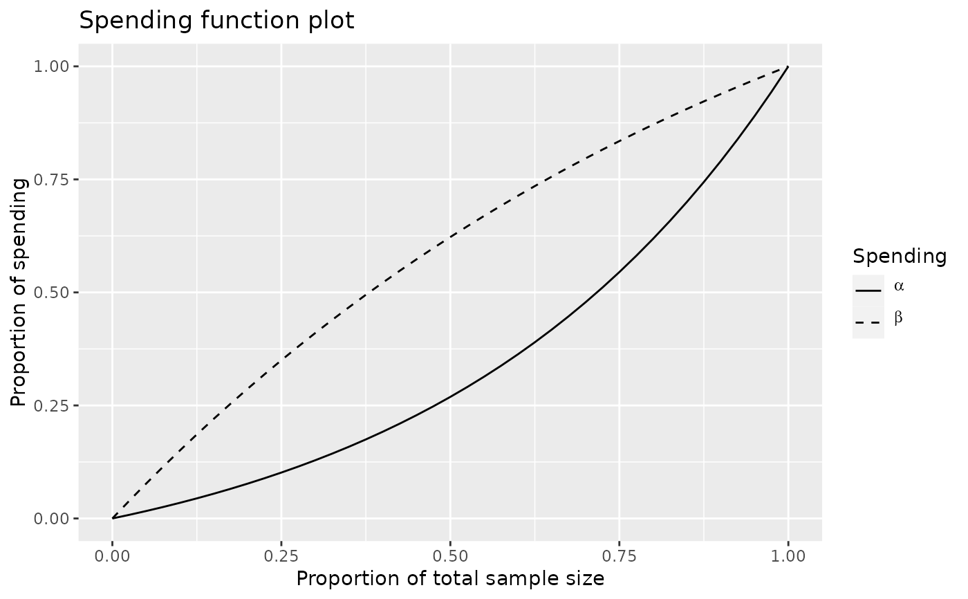
# plot the alpha- and beta-spending functions
plot(x, plottype=5)


# what happens to summary if we used a boundary function design
x <- gsDesign(test.type=2,sfu="OF")
y <- gsDesign(test.type=1,sfu="WT",sfupar=.25)
summary(x$upper)
#> [1] "O'Brien-Fleming boundary"
summary(y$upper)
#> [1] "Wang-Tsiatis boundary with Delta = 0.25"

# Example 2: advanced example: writing a new spending function  
# Most users may ignore this!

# implementation of 2-parameter version of
# beta distribution spending function
# assumes t and alpha are appropriately specified (does not check!) 
sfbdist <- function(alpha,  t,  param)
{  
   # check inputs
   checkVector(param, "numeric", c(0, Inf), c(FALSE, TRUE))
   if (length(param) !=2) stop(
   "b-dist example spending function parameter must be of length 2")

   # set spending using cumulative beta distribution and return
   x <- list(name="B-dist example", param=param, parname=c("a", "b"), 
             sf=sfbdist, spend=alpha * 
           pbeta(t, param[1], param[2]), bound=NULL, prob=NULL)  
           
   class(x) <- "spendfn"
   
   x
}

# now try it out!
# plot some example beta (lower bound) spending functions using 
# the beta distribution spending function 
t <- 0:100/100
plot(t, sfbdist(1, t, c(2, 1))$spend, type="l", 
    xlab="Proportion of information", 
    ylab="Cumulative proportion of total spending", 
    main="Beta distribution Spending Function Example")
lines(t, sfbdist(1, t, c(6, 4))$spend, lty=2)
lines(t, sfbdist(1, t, c(.5, .5))$spend, lty=3)
lines(t, sfbdist(1, t, c(.6, 2))$spend, lty=4)
legend(x=c(.65, 1), y=1 * c(0, .25), lty=1:4, 
    legend=c("a=2, b=1","a=6, b=4","a=0.5, b=0.5","a=0.6, b=2"))