Group sequential design interim density function

Given an interim analysis i of a group sequential design and a vector of real values zi, gsDensity() computes an interim density function at analysis i at the values in zi. For each value in zi, this interim density is the derivative of the probability that the group sequential trial does not cross a boundary prior to the i-th analysis and at the i-th analysis the interim Z-statistic is less than that value. When integrated over the real line, this density computes the probability of not crossing a bound at a previous analysis. It corresponds to the subdistribution function at analysis i that excludes the probability of crossing a bound at an earlier analysis.

The initial purpose of this routine was as a component needed to compute the predictive power for a trial given an interim result; see gsPP.

See Jennison and Turnbull (2000) for details on how these computations are performed.

Usage

gsDensity(x, theta = 0, i = 1, zi = 0, r = 18)

Arguments

x: An object of type gsDesign or gsProbability
theta: a vector with $\theta$ value(s) at which the interim density function is to be computed.
i: analysis at which interim z-values are given; must be from 1 to x$k
zi: interim z-value at analysis i (scalar)
r: Integer value (>= 1 and <= 80) controlling the number of numerical integration grid points. Default is 18, as recommended by Jennison and Turnbull (2000). Grid points are spread out in the tails for accurate probability calculations. Larger values provide more grid points and greater accuracy but slow down computation. Jennison and Turnbull (p. 350) note an accuracy of $10^{-6}$ with r = 16. This parameter is normally not changed by users.

Value

zi: The input vector zi.
theta: The input vector theta.
density: A matrix with length(zi) rows and length(theta) columns. The subdensity function for z[j], theta[m] at analysis i is returned in density[j,m].

Note

The gsDesign technical manual is available at https://keaven.github.io/gsd-tech-manual/.

References

Jennison C and Turnbull BW (2000), Group Sequential Methods with Applications to Clinical Trials. Boca Raton: Chapman and Hall.

Author

Keaven Anderson keaven_anderson@merck.com

Examples

library(ggplot2)
# set up a group sequential design
x <- gsDesign()

# set theta values where density is to be evaluated
theta <- x$theta[2] * c(0, .5, 1, 1.5)

# set zi values from -1 to 7 where density is to be evaluated
zi <- seq(-3, 7, .05)

# compute subdensity values at analysis 2
y <- gsDensity(x, theta = theta, i = 2, zi = zi)

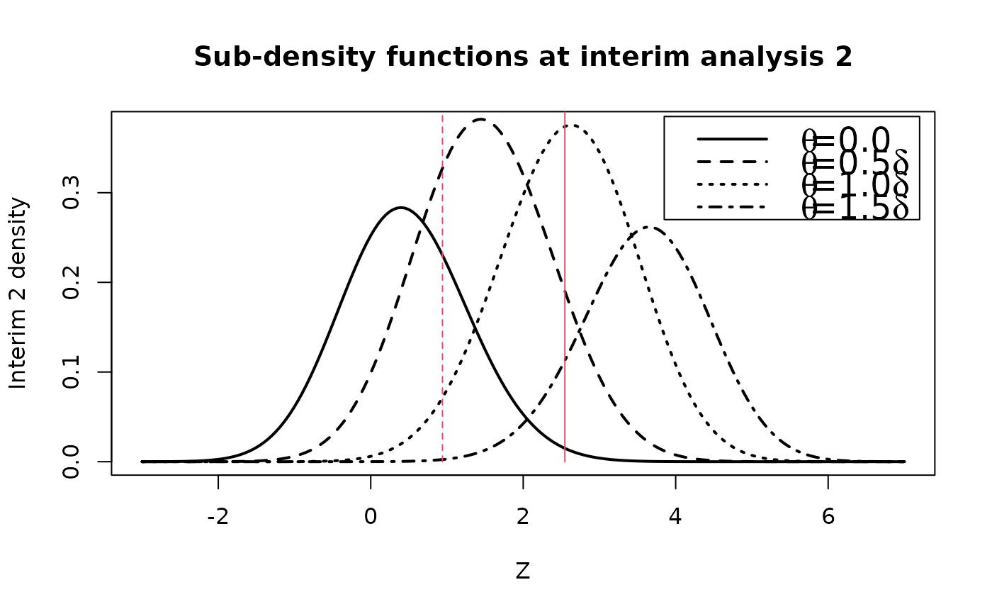
# plot sub-density function for each theta value
plot(y$zi, y$density[, 3],
  type = "l", xlab = "Z",
  ylab = "Interim 2 density", lty = 3, lwd = 2
)
lines(y$zi, y$density[, 2], lty = 2, lwd = 2)
lines(y$zi, y$density[, 1], lwd = 2)
lines(y$zi, y$density[, 4], lty = 4, lwd = 2)
title("Sub-density functions at interim analysis 2")
legend(
  x = c(3.85, 7.2), y = c(.27, .385), lty = 1:5, lwd = 2, cex = 1.5,
  legend = c(
    expression(paste(theta, "=0.0")),
    expression(paste(theta, "=0.5", delta)),
    expression(paste(theta, "=1.0", delta)),
    expression(paste(theta, "=1.5", delta))
  )
)

# add vertical lines with lower and upper bounds at analysis 2
# to demonstrate how likely it is to continue, stop for futility
# or stop for efficacy at analysis 2 by treatment effect
lines(rep(x$upper$bound[2], 2), c(0, .4), col = 2)
lines(rep(x$lower$bound[2], 2), c(0, .4), lty = 2, col = 2)


# Replicate part of figures 8.1 and 8.2 of Jennison and Turnbull text book
# O'Brien-Fleming design with four analyses

x <- gsDesign(k = 4, test.type = 2, sfu = "OF", alpha = .1, beta = .2)

z <- seq(-4.2, 4.2, .05)
d <- gsDensity(x = x, theta = x$theta, i = 4, zi = z)

plot(z, d$density[, 1], type = "l", lwd = 2, ylab = expression(paste(p[4], "(z,", theta, ")")))
lines(z, d$density[, 2], lty = 2, lwd = 2)
u <- x$upper$bound[4]
text(expression(paste(theta, "=", delta)), x = 2.2, y = .2, cex = 1.5)
text(expression(paste(theta, "=0")), x = .55, y = .4, cex = 1.5)