Spending Function

Spending Function

Usage

# S3 method for spendfn
summary(object, ...)

spendingFunction(alpha, t, param)

Arguments

object: A spendfn object to be summarized.
...: Not currently used.
alpha: Real value \(> 0\) and no more than 1. Defaults in calls to gsDesign() are alpha=0.025 for one-sided Type I error specification and alpha=0.1 for Type II error specification. However, this could be set to 1 if, for descriptive purposes, you wish to see the proportion of spending as a function of the proportion of sample size/information.
t: A vector of points with increasing values from 0 to 1, inclusive. Values of the proportion of sample size/information for which the spending function will be computed.
param: A single real value or a vector of real values specifying the spending function parameter(s); this must be appropriately matched to the spending function specified.

Value

spendingFunction and spending functions in general produce an object of type spendfn.

name: A character string with the name of the spending function.
param: any parameters used for the spending function.
parname: a character string or strings with the name(s) of the parameter(s) in param.
sf: the spending function specified.
spend: a vector of cumulative spending values corresponding to the input values in t.
bound: this is null when returned from the spending function, but is set in gsDesign() if the spending function is called from there. Contains z-values for bounds of a design.
prob: this is null when returned from the spending function, but is set in gsDesign() if the spending function is called from there. Contains probabilities of boundary crossing at i-th analysis for j-th theta value input to gsDesign() in prob[i,j].

Note

The gsDesign technical manual is available at https://keaven.github.io/gsd-tech-manual/.

References

Jennison C and Turnbull BW (2000), Group Sequential Methods with Applications to Clinical Trials. Boca Raton: Chapman and Hall.

Author

Keaven Anderson keaven_anderson@merck.com

Examples

# Example 1: simple example showing what most users need to know

# Design a 4-analysis trial using a Hwang-Shih-DeCani spending function
# for both lower and upper bounds
x <- gsDesign(k = 4, sfu = sfHSD, sfupar = -2, sfl = sfHSD, sflpar = 1)

# Print the design
x
#> Asymmetric two-sided group sequential design with
#> 90 % power and 2.5 % Type I Error.
#> Upper bound spending computations assume
#> trial continues if lower bound is crossed.
#> 
#>            Sample
#>             Size   ----Lower bounds----  ----Upper bounds-----
#>   Analysis Ratio*  Z   Nominal p Spend+  Z   Nominal p Spend++
#>          1  0.324 0.03    0.5136 0.0350 2.80    0.0025  0.0025
#>          2  0.649 0.88    0.8096 0.0273 2.58    0.0049  0.0042
#>          3  0.973 1.51    0.9349 0.0212 2.34    0.0096  0.0069
#>          4  1.297 2.09    0.9817 0.0165 2.09    0.0183  0.0114
#>      Total                       0.1000                 0.0250 
#> + lower bound beta spending (under H1):
#>  Hwang-Shih-DeCani spending function with gamma = 1.
#> ++ alpha spending:
#>  Hwang-Shih-DeCani spending function with gamma = -2.
#> * Sample size ratio compared to fixed design with no interim
#> 
#> Boundary crossing probabilities and expected sample size
#> assume any cross stops the trial
#> 
#> Upper boundary (power or Type I Error)
#>           Analysis
#>    Theta      1      2      3      4  Total   E{N}
#>   0.0000 0.0025 0.0042 0.0065 0.0072 0.0203 0.5477
#>   3.2415 0.1695 0.3553 0.2774 0.0978 0.9000 0.7533
#> 
#> Lower boundary (futility or Type II Error)
#>           Analysis
#>    Theta      1      2      3      4  Total
#>   0.0000 0.5136 0.3156 0.1169 0.0336 0.9797
#>   3.2415 0.0350 0.0273 0.0212 0.0165 0.1000
# Summarize the spending functions
summary(x$upper)
#> [1] "Hwang-Shih-DeCani spending function with gamma = -2"
summary(x$lower)
#> [1] "Hwang-Shih-DeCani spending function with gamma = 1"

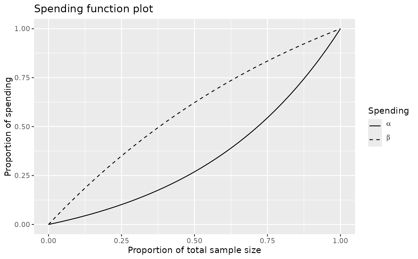
# Plot the alpha- and beta-spending functions
plot(x, plottype = 5)


# What happens to summary if we used a boundary function design
x <- gsDesign(test.type = 2, sfu = "OF")
y <- gsDesign(test.type = 1, sfu = "WT", sfupar = .25)
summary(x$upper)
#> [1] "O'Brien-Fleming boundary"
summary(y$upper)
#> [1] "Wang-Tsiatis boundary with Delta = 0.25"

# Example 2: advanced example: writing a new spending function
# Most users may ignore this!

# Implementation of 2-parameter version of
# beta distribution spending function
# assumes t and alpha are appropriately specified (does not check!)
sfbdist <- function(alpha, t, param) {
  # Check inputs
  checkVector(param, "numeric", c(0, Inf), c(FALSE, TRUE))
  if (length(param) != 2) {
    stop(
      "b-dist example spending function parameter must be of length 2"
    )
  }

  # Set spending using cumulative beta distribution and return
  x <- list(
    name = "B-dist example", param = param, parname = c("a", "b"),
    sf = sfbdist, spend = alpha *
      pbeta(t, param[1], param[2]), bound = NULL, prob = NULL
  )

  class(x) <- "spendfn"

  x
}

# Now try it out!
# Plot some example beta (lower bound) spending functions using
# the beta distribution spending function
t <- 0:100 / 100
plot(
  t, sfbdist(1, t, c(2, 1))$spend,
  type = "l",
  xlab = "Proportion of information",
  ylab = "Cumulative proportion of total spending",
  main = "Beta distribution Spending Function Example"
)
lines(t, sfbdist(1, t, c(6, 4))$spend, lty = 2)
lines(t, sfbdist(1, t, c(.5, .5))$spend, lty = 3)
lines(t, sfbdist(1, t, c(.6, 2))$spend, lty = 4)
legend(
  x = c(.65, 1), y = 1 * c(0, .25), lty = 1:4,
  legend = c("a=2, b=1", "a=6, b=4", "a=0.5, b=0.5", "a=0.6, b=2")
)