1 Background

1.1 Non-proportional hazards

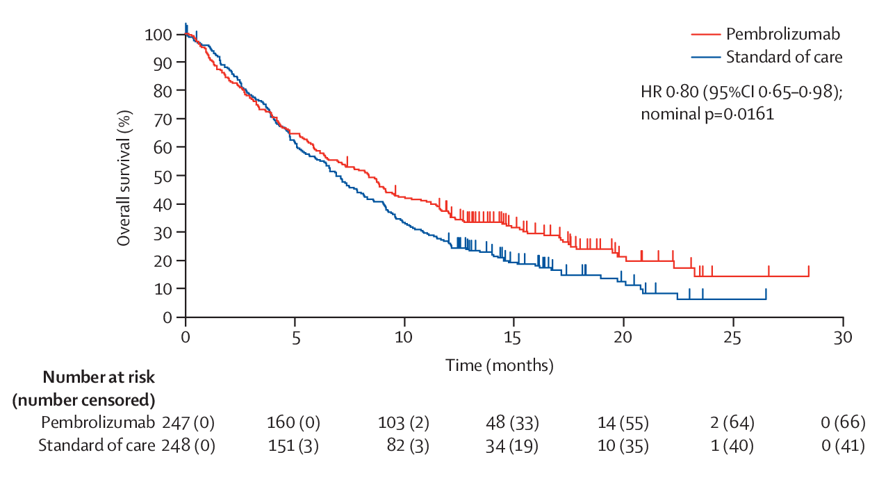
Non-proportional hazards (NPH) are very common to see when there is a delayed effect. One example is given by KEYNOTE040, which targets to cure recurrent head and neck squamous cell carcinoma. There are two arms, one is pembrolizumab, and the other is standard of care (SOC). The randomization ratio is 1:1 and the total sample size is 495. The primary endpoint is overall survival (OS) with 90% power for HR=0.7, 1-sided \(\alpha=0.025\) (The detailed design can be referred to the protocol).

There are two interim analysis planned, one at 144 deaths (with information fraction as 0.42) and the other at 216 deaths (with information fraction as 0.64). The efficacy boundary is Hwang-Shih-DeCani (HSD) spending with \(\gamma=-4\), and the futility boundary is non-binding \(\beta\)-spending HSD with \(\gamma = -16\). The final analysis finds there are 388 deaths, compared with 340 planned death. The 1-sided nominal p-value for OS at the final analysis is 0.0161.

FIGURE 1.1: KEYNOTE040

From the figure above, we can see there is a delay of the treatment effect.

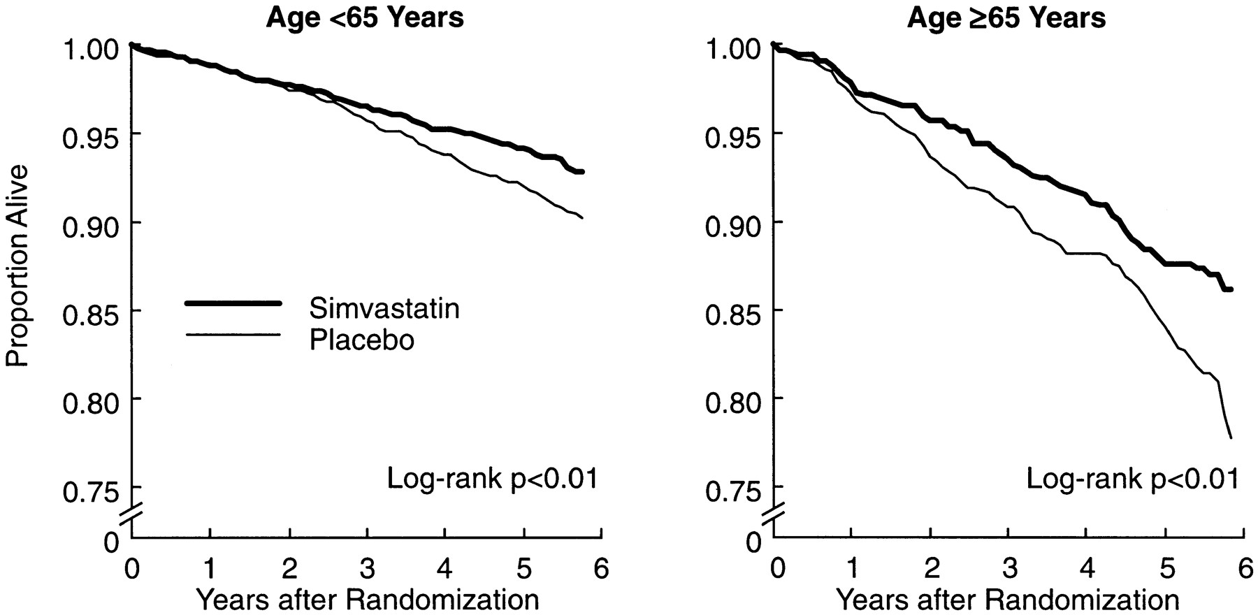
The delayed effect is not just in oncology, it also lies in other TA. For example, in cholesterol lowering and mortality (Miettinen et al 1997), there is also a delayed effect.

FIGURE 1.2: Scandinavian Simvastatin Survival Study

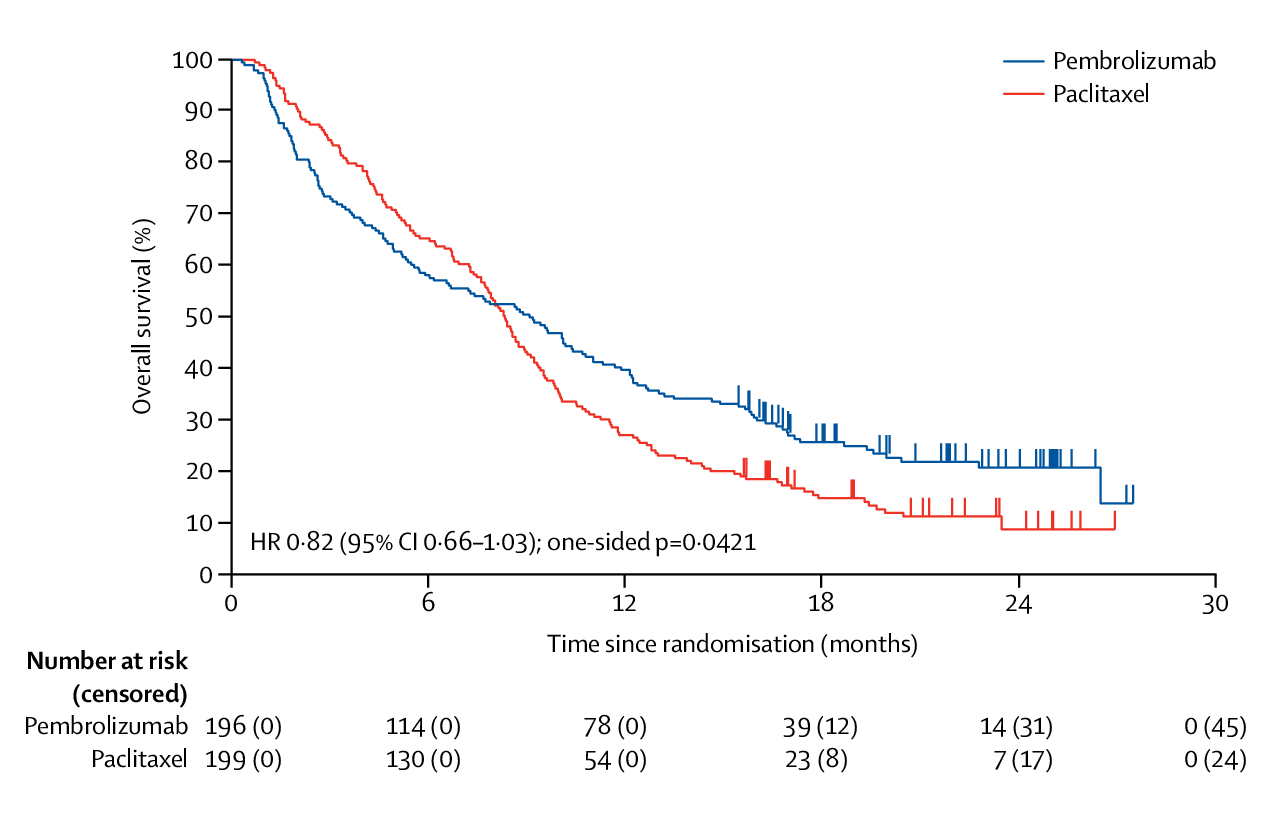
In addition to delayed effect, NPH also exists when there is a cross over of survival curves. For example, in KEYNOTE061 (recurrent advanced gastric or gastro-oesophageal junction cancer), there is a cross over of the pembrolizumab arm and paclitaxel arm (see figure below). It is 1:1 randomization with 360 planned events (395 actual events) at the end of the trial in CPS \(\ge\) 1 population. The first primary endpoints is OS in PD-L1 CPS \(\ge\) 1. Its power is 91% for HR=0.67 with 1-sided \(\alpha=0.0215\). The secondary primary endpoints is PFS in PD-L1 CPS \(\ge\) 1. (The detailed design can be found in the protocol

When it proceeded to final analysis, there are 326 deaths with 290 planned. One interim analysis is conducted with 240 events at information fraction of 0.83. During the group sequential design, the efficacy boundary is Hwang-Shih-DeCani (HSD) spending with \(\gamma=-4\) and there is not a futility boundary. The 1-sided nominal p-value for OS is 0.0421 (threshold: p=0.0135). And Post hoc FH(\(\rho=1,\gamma=1\)) is p=0.0009.

KEYNOTE 061: Overall Survival in CPS 1

FIGURE 1.3: KEYNOTE061

The above two examples motivate us to think about the following questions:

• The impact of (potentially) delayed treatment effect on trial design and analysis.
• Test statistics used (logrank, weighted logrank test, and max-combo test)
• Sample size vs. duration of follow-up
• Timing of analyses
• Futility bounds
• Updating bounds
• Multiplicity adjustments

1.1.1 Group sequential design

In group sequential design, groups of observations are collected and repeatedly analyzed, while controlling error rates. While the group sequential design is ongoing, a stopping rule specifies when and why a trial might be halted at these points. This stopping rule usually consists of two components, a test statistic and a threshold. The threshold is usually decided by the spending functions, which we introduced in Section 1.2. And the test statistics are usually the Z-process and B-process, which are used to monitor the treatment effect under group sequential design. If a Z-process (B-process) cross the boundary, the trial is stopped.

1.1.2 Z-process and B-process

In this section, we will introduce the Z-process and B-process. Suppose in the group sequential design, there are totally \(K\) looks. In the \(k\)-th look, there are \(n_k\) available observations. For notation simplicity, we denote the final number of available observations as \(N\), i.e., \(N \triangleq n_K\).

Definition 1.1 The Z-process is defined as the standardized treatment effect, i.e., \[\begin{equation} Z_{k} = \frac{\widehat\theta_k}{\sqrt{\hbox{Var}(\hat\theta_k)}}, \tag{1.1} \end{equation}\] where \(k\) is the index of the looks, and we assume there are totally \(K\) number of looks, i.e., \(k = 1, 2, \ldots, K\). The numerator \(\widehat\theta_k\) is the treatment effect estimated at the \(k\)-th look.

For \(\widehat\theta_k\), its form depends on the outcome of the clinical trials. In clinical trials with continuous outcome \(X_1, X_2, \ldots \in \mathbb R\), the treatment effect estimated at the \(k\)-th look is \[\begin{equation} \widehat{\theta}_k = \frac{\sum_{i=1}^{n_k} X_{i}}{n_k}\equiv \bar X_{k}, \tag{1.2} \end{equation}\] where \(n_k\) is the number of available observations at the \(k\)-th look. In clinical trials with binary outcome \(X_1, X_2, \ldots \in \mathbb \{0, 1\}\), \(\widehat\theta_k\) can be estimated the same as in equation (1.2). In clinical trials with survival outcome, \(\widehat\theta_k\) would typically represent a Cox model coefficient representing the logarithm of the hazard ratio for experimental vs. control treatment. And \(n_k\) would represent the planned number of events at \(k\)-th look.

After discussing the Z-process, let us take a look at the B-process.

Definition 1.2 The B-process is defined as \[\begin{equation} B_{k} = \sqrt{t_k} Z_k, \tag{1.3} \end{equation}\] where \(Z_k\) is defined in Definition 1.1 and \(t_k\) is the information fraction at the \(k\)-th look, i.e., \[ t_k = \mathcal I_k / \mathcal I_K, \] where \(\mathcal I_k\) is the information at the \(k\)-th look, defined as \[ \mathcal I_k \triangleq \frac{1}{\text{Var}(\widehat\theta_k)}. \]

The information sequence plays an important role in the group sequential design. For example, in a clinical trial with continuous outcome \(X_1, X_2, \ldots \overset{i.i.d.}{\sim} N(\mu, \sigma^2)\), the information at the \(k\)-th look is \(\mathcal I_k = n_k\) with \(n_k\) as the number of available observations at the \(k\)-th look. The same logic applies to the binary outcome. Another example is a clinical trial with survival outcome. In this case, the information at the \(k\)-th look is \(\mathcal I_k = n_k\) with \(n_k\) as the number of events at the \(k\)-th look.

1.1.3 Canonical form

In the group sequential design, given the total \(K\) look, there are sequences of Z-process and B-process, i.e., \(\{Z_k\}_{k = 1, \ldots, K}\) and \(\{B_k\}_{k = 1, \ldots, K}\). The CF refers to the joint distribution of \(\{Z_k\}_{k = 1, \ldots, K}\) and \(\{B_k\}_{k = 1, \ldots, K}\), including the distribution, the expectation mean, variance and covariance. Please note that this distribution is asymptotic, and the asymptotic conditions usually requires the sample size to be relative large. Properly speaking, both \(\{Z_k\}_{k = 1, \ldots, K}\) and \(\{B_k\}_{k = 1, \ldots, K}\) depends on the sample size, which can be re-denoted as \(\{ Z_{k,N} \}_{k = 1, \ldots, K}\) and \(\{ B_{k, N} \}_{k = 1, \ldots, K}\). When the sample size is relatively large, we can get rid of the sample size, i.e., \[ Z_k = \lim\limits_{N \to \infty} Z_{k,N}. \] This asymptotic assumed throughout this book.

An important assumption of CF is \(E(\widehat\theta_k) = \theta\), where \(\theta\) is a constant and \(\widehat\theta\) is defined in equation (1.2).

Theorem 1.1 Suppose in a group sequential design, there are totally \(K\) looks. At the \(k\)-th look, there are \(n_k\) available observations, i.e., \(\{X_i\}_{i = 1, \ldots, n_k}\). Assume that \(\text{Var}(X_i) = 1\) for \(i = 1, 2, \ldots, N\). And denote \(\mathcal I_k \triangleq \frac{1}{\text{Var}(\widehat\theta(t_k))}\) and \(E(\widehat\theta_k) = \theta\). The joint distribution of Z-process \(\{Z_k\}_{k = 1, \ldots, K}\) is \[ \left\{ \begin{array}{l} (Z_1, \ldots, Z_K) \text{ is multivariate normal} \\ E(Z_k) = \sqrt{\mathcal{I}_k}\theta \\ \hbox{Var}(Z_k) = 1 \\ \text{Cov}(Z_i, Z_j) = \sqrt{t_i/t_j} \;\; \forall 1 \leq i \leq j \leq K \end{array} \right.. \] where \(t_i = n_i / N\) with \(N \triangleq n_K\) as the final number of observations at the last look. If a statistics have the above distribution, we declare that it has the canonical joint distribution with information levels \(\{\mathcal I_1, \ldots, \mathcal I_K \}\) for the parameter \(\theta\).

From the above theorem, we found that CF treats \(E(\widehat\theta)\) as a constant, i.e., \(\theta\). Following the similar, we can also summarize the distribution of B-process.

Theorem 1.2 Following the same setting of Theorem 1.1 The distribution of B-process is \[ \left\{ \begin{array}{l} (B_1, \ldots, B_K) \text{ is multivariate normal} \\ E(B_k) = \sqrt{t_{k}\mathcal{I}_k}\theta = t_k \sqrt{\mathcal{I}_K} \theta = \mathcal{I}_k \theta / \sqrt{\mathcal{I}_K} \\ \hbox{Var}(B_k) = t_k \\ \text{Cov}(B_i, B_j) = t_i \;\; \forall 1 \leq i \leq j \leq K \end{array} \right., \] where \(t_i = n_i/N\) with \(N \triangleq n_K\) as the final number of observations at the last look.

It should be noted that the correlation of B-process is the same as the covariance of Z-process, i.e., \[\begin{equation} Corr(B_i, B_j) = Cov(Z_i, Z_j) = \sqrt{t_i/t_j} \;\; \forall 1 \leq i \leq j \leq K. \end{equation}\] To learn this covariance/correlation better, let us take the continuous outcome as an example. Suppose there are \(K\) looks in a clinical trial, and at the \(k\)-th look, there are \(n_k\) available observations with outcome \(\{ X_i \}_{i = 1, \ldots, n_k}\). In this example, we have \[\begin{eqnarray} B_k & = & \sqrt{t_k} Z_k = \sqrt{\mathcal I_k / \mathcal I_K} \frac{\widehat\theta_k}{\sqrt{Var(\widehat\theta_k)}} = \mathcal I_k\sqrt{ 1 / \mathcal I_K} \widehat\theta_k \\ & = & \mathcal I_k\sqrt{ 1 / \mathcal I_K} \frac{\sum_{i=1}^{n_k} X_i}{n_k} = \frac{\sum_{i=1}^{n_k} X_i}{\sqrt{I_K}} = \frac{\sum_{i=1}^{n_k} X_i}{\sqrt{N}}. \end{eqnarray}\] Given the above B-process, for any \(1 \leq i \leq j \leq K\), we have \[ B_j - B_i \sim N(\mathcal I_j \theta(t_j) - \mathcal I_i \theta(t_i), t_j - t_i) \] independent of \(B_1, B_2, \ldots, B_i\). So we have \[\begin{eqnarray} Corr(B_i, B_j) & = & Cov(B_i, B_j) \bigg / \sqrt{Var(B_i) Var(B_j)} \\ & = & t_i \bigg / \sqrt{t_i t_j} = \sqrt{t_i / t_j} \\ & = & Cov(Z_i, Z_j) \end{eqnarray}\]

1.1.4 Extended canonical form

The main difference between extended canonical form (ECF) and canonical form (CF) is that, ECF treats \(E(\widehat\theta_k)\) as a time-varying parameter, i.e., \(\theta(t_k)\). While CF treats it as a constant \(\theta\). So we summarize the joint distribution of Z-process and B-process under ECF as follows

Theorem 1.1 Suppose in a group sequential design, there are totally \(K\) looks. At the \(k\)-th look, there are \(n_k\) available observations, i.e., \(\{X_i\}_{i = 1, \ldots, n_k}\). Assume that \(\text{Var}(X_i) = 1\) for \(i = 1, 2, \ldots, N\). And denote \(\mathcal I_k \triangleq \frac{1}{\text{Var}(\widehat\theta(t_k))}\) and \(E(\widehat\theta_k) = \theta(t_k)\). The joint distribution of Z-process \(\{Z_k\}_{k = 1, \ldots, K}\) is \[ \left\{ \begin{array}{l} (Z_1, \ldots, Z_K) \text{ is multivariate normal} \\ E(Z_k) = \sqrt{\mathcal{I}_k} \theta(t_k) \\ \hbox{Var}(Z_k) = 1 \\ \text{Cov}(Z_i, Z_j) = \sqrt{t_i/t_j} \;\; \forall 1 \leq i \leq j \leq K \end{array} \right.. \] And the joint distribution of B-process \(\{B_k\}_{k = 1, \ldots, K}\) is \[ \left\{ \begin{array}{l} (B_1, \ldots, B_K) \text{ is multivariate normal} \\ E(B_k) = \sqrt{t_{k}\mathcal{I}_k}\theta(t_k) = t_k \sqrt{\mathcal{I}_K} \theta(t_k) = \mathcal{I}_k\theta(t_k)/\sqrt{\mathcal{I}_K}\\ \hbox{Var}(B_k) = t_k \\ \text{Cov}(B_i, B_j) = t_i \;\; \forall 1 \leq i \leq j \leq K \end{array} \right., \] where \(t_i = n_i / N\) with \(N \triangleq n_K\) as the final number of observations at the last look. If a statistics have the above distribution, we declare that it has the canonical joint distribution with information levels \(\{\mathcal I_1, \ldots, \mathcal I_K \}\) for the parameter \(\theta\).

1.2 Spending function bounds

In this section, we introduce the spending function bounds in group sequential design. We start with it definitions and categories. And then introduce three frequently used spending functions, (1) Haybittle boundary, (2) Pocock boundary and (3) O’Brien-Fleming boundary.

Suppose we have \(K\) analyses conducted at information fraction of \(t_1, t_2, \ldots, t_k, \ldots, t_K\). We call the \(\{a_k, b_k \}_{k = 1,\ldots, K}\) as the decision boundaries, if we reject \(H_0\) when \(Z(t_k) < a_k\) or \(Z(t_k) > b_k\). And we call \(\{b_k\}_{k=1,\ldots,K}\) as the efficiency boundary, which are decided by the control of type I error, and \(\{a_k\}_{k=1,\ldots,K}\) as the futility boundary, which are used to control boundary crossing probabilities.

For the calculation of boundaries, there are typically two methods. The first one is the so-called error spending approach, which specifies boundary crossing probabilities at each analysis. This is most commonly done with the error spending function approach (Lan and DeMets 1983). The second one is the so-called boundary family approach, which specifies how big boundary values should be relative to each other and adjust these relative values by a constant multiple to control overall error rates. The commonly applied boundary family include:

• Haybittle boundary (Haybittle 1971);
• Wang-Tsiatis boundary (Wang and Tsiatis 1987):
  • Pocock boundary (Pocock 1977);
  • O’Brien and Fleming boundary (O’Brien and Fleming 1979).

In the remainder of this section, we will introduce the above spending functions one by one.

1.2.1 Haybittle boundary

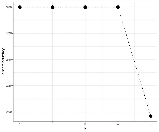
The main idea of the Haybittle boundary is to set the interim Z-score boundary as 3 and the final boundary as 1.96, which is visualized in the figure below.

FIGURE 1.4: Haybittle boundary

The above Haybittle boundary has three modified versions.

The first modified version uses Bonferroni adjustment: for the first \(K-1\) analyses, the significant p-value is set as 0.001; and for the final analysis, the significant p-value is set as \(0.05 - 0.01 \times (K-1)\). This modification helps to avoid type I error inflation. Besides, it does not require them to be equally spaced in terms of information and can be used regardless of the joint distribution of Z-score, i.e., \(Z(t_1),...,Z(t_k)\).

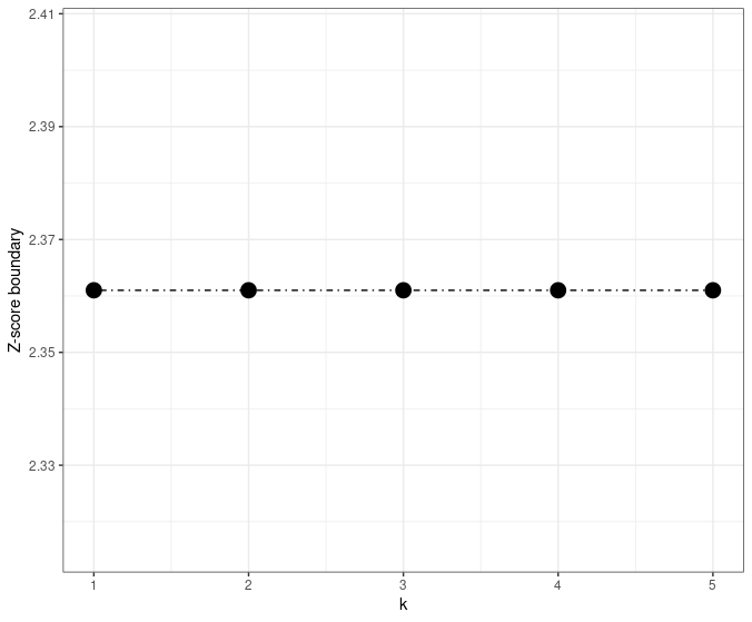
The second modified version sets the Z-score as 4 for the first half of the study and sets the Z-score boundary as 3 thereafter.

The third modified version requires crossing the boundary at two successive looks.

In summary, the Haybittle boundary uses a piecewise constant boundary, which makes it very easy to implement. But it is kind of conservative, and the selection of the constant boundary (e.g., 3 and 1.96) needs justifications.

1.2.2 Wang-Tsiatis boundary

For 2-sided testing, Wang and Tsiatis (1987) defined the boundary function for the \(k\)-th look as \[ \Gamma(\alpha, K, \Delta) k^{\Delta - 0.5}, \] where \(\Gamma(\alpha, K, \Delta)\) is a constant chosen so that the level of significance is equal to \(\alpha\).

With two selection of \(\Delta\), the Wang-Tsiatis boundary gives two special cases. When \(\Delta = 0.5\), it is the Pocock bounds. When \(\Delta = 0\), it is the O’Brien-Fleming bounds.

1.2.3 Pocock boundary

For 2-sided testing, the Pocock procedure rejects at the \(k\)-th of \(K\) looks if \[ |Z(k/K)| > c_P(K), \] where \(c_P(K)\) is fixed given the number of total looks \(K\) and chosen such that \(\text{Pr}(\cup_{k=1}^{K} |Z(k/K)| > c_P(K)) = \alpha\).

FIGURE 1.5: Pocock boundary

Here is an example of the Pocock boundary.

total number of looks(K)	\(\alpha = 0.01\)	\(\alpha = 0.05\)	\(\alpha = 0.1\)
1	2.576	1.960	1.645
2	2.772	2.178	1.875
4	2.939	2.361	2.067
8	3.078	2.512	2.225
\(\infty\)	\(\infty\)	\(\infty\)	\(\infty\)

We will reject \(H_0\) if \(|Z(k/4)| > 2.361\) for \(k = 1,2,3,4\) (final analysis).

In summary, the Pocock boundary is a special case of Wang-Tsiatis boundary (\(\Delta = 0.5\)) and has constant Z-score boundaries, i.e., \(|Z(k/K)| > c_P(K)\). And the constant boundary \(c_P(K)\) is decided by the type I error rate and the total number of looks. Its main weakness is the high price for the end of the trial and the requirement of equally spaced looks.

1.2.4 O’Brien-Fleming boundary

O’Brien-Fleming boundary is very conservative at the beginning, which gives a relatively large boundary first. But it gives a nominal value close to the overall value of the design \(\approx 1.96\) when two-sied \(\alpha = 0.05\) for the final stage. Its visualization can be found as follows.

FIGURE 1.6: OBrien-Fleming boundary

Here is an example of the O’Brien-Fleming boundary.

total number of looks(K)	\(\alpha = 0.01\)	\(\alpha = 0.05\)	\(\alpha = 0.1\)
1	2.576	1.960	1.645
2	2.580	1.977	1.678
4	2.609	2.024	1.733
8	2.648	2.072	1.786
16	2.684	2.114	1.830
\(\infty\)	2.807	2.241	1.960

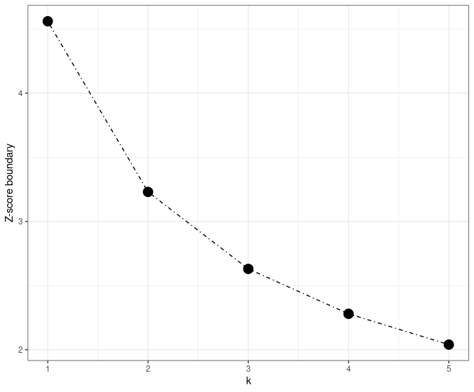
Since the tabled value 2.024 is the flat B-value boundary. The B-value boundary can be easily transformed into decreasing Z-score boundary by \(Z(t) = B(t)/\sqrt{t}\):

• \(2.024/\sqrt{1/4} = 4.05\)
• \(2.024/\sqrt{2/4} = 2.86\)
• \(2.024/\sqrt{3/4} = 2.34\)
• \(2.024/\sqrt{4/4} = 2.02\)

In summary, the O’Brien-Fleming boundary designs a decreasing Z-score boundary, with large boundaries at the early stage but ~1.96 boundary when it approaches the final stage.

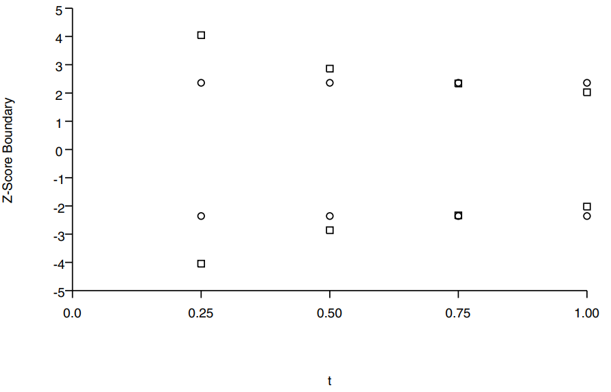
Although both the Pocock boundary and OBF boundary belong to the Wang-Tsiatis boundary’s family, there are two differences between them.

The first difference is, the Pocock boundary has flat Z-score boundaries, while the O’Brien-Fleming has decreasing Z-score boundary. Accordingly, the O’Brien-Fleming boundary makes it much more difficult to stop early than the Pocock boundary. However, the O’Brien-Fleming boundary extracts a much smaller price at the end.

FIGURE 1.7: Pocock (circles) and O’Brien-Fleming (squares) z-score boundaries for four looks

The second difference is, they have different performance in cumulative type I error rate (the probability of rejection at or before \(t_j\), i.e., \(\text{Pr}(\cup_{i=1}^j |Z(t_i)| > c_i)\)).

• The Pocock cumulative type I error rate increases sharply at first, but much less so toward the end.
• The O’Brien-Fleming behaves in just the opposite way.

FIGURE 1.8: Cumulative type I error rate used by the Pocock (circles) and O’Brien-Fleming (squares) procedures with four looks.

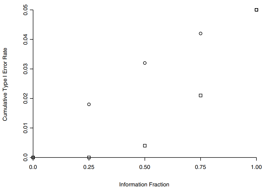
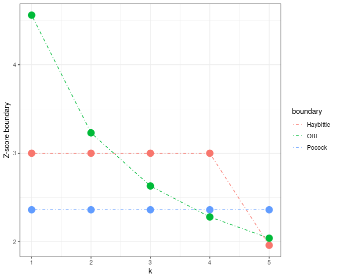
In conclusion, we visualize the three spending functions in the following figure.

FIGURE 1.9: Three boundaries

1.3 Statistical information and time

Statistical information and time is a key component in group sequential design. In this section, we introduce the statistical information under three different outcomes, (1) continuous outcome, (2) binary outcome and (3) survival outcome.

We start with the continuous outcome. Suppose in a \(T\)-month trial, and the interim analysis is conducted after \(\tau\) month with \(n\) of \(N\) planned observations evaluated in each arm. These \(n\) available observation is denoted as \(\{X_i\}_{i = 1, \ldots, n}\) for the control arm and \(\{Y_i\}_{i = 1, \ldots, n}\) for the treatment arm. Thus, the treatment effect can be estimated as \[ \widehat\delta(\tau) = \frac{\sum_{i=1}^n (Y_i - X_i)}{n}. \] For \(Y_i - X_i\), we commonly assume that \(Y_i - X_i \overset{i.i.d.}{\sim} \text{Normal}(\mu, \sigma^2)\) for any \(i = 1, \ldots, n\), with \(\mu = 0\) under the null hypothesis and \(\mu \neq 0\) under the alternative hypothesis.

The information at the \(\tau\)-th month is \[ I(\tau) = 1/\text{Var}(\widehat\delta(\tau)) = n/\sigma^2. \] Accordingly, we define the information fraction as the ratio between interim information and final information, i.e., \[ t = I(\tau)/I(T)= \frac{n/\sigma^2}{N/\sigma^2} = \frac{n}{N}. \]

For binary outcome, it follows the similar logic as that in continuous outcome. We commonly assume that \(Y_i - X_i \overset{i.i.d.}{\sim} \text{Bernoulli}(p)\) for any \(i = 1, \ldots, n\), with \(p = 0.5\) under the null hypothesis and \(p \neq 0.5\) under the alternative hypothesis. The information at the \(\tau\)-th month is \[ I(\tau) = 1/\text{Var}(\widehat\delta(\tau)) = \frac{n}{p(1-p)}. \] Accordingly, the information fraction is \[ t = I(\tau)/I(T)= \frac{\frac{n}{p(1-p)}}{\frac{N}{p(1-p)}} = \frac{n}{N}. \]

For survival outcome, it is a little bit complicated. Suppose the interim analysis is conducted after \(\tau\) month with \(d\) of \(D\) planned events evaluated in each arm. The treatment effect under survival outcome is usually measured by logrank test, i.e., \[ \widehat\delta(\tau) = \frac{\sum_{i=1}^d (O_i - E_i)}{\sum_{i = 1}^d V_i} \triangleq \frac{S(\tau)}{\sum_{i = 1}^d V_i}. \] Accordingly, the information fraction is \[ \begin{array}{ccl} t & = & \text{Var}(S(\tau)) / \text{Var}(S(1)) \\ & = & \text{Var}(\sum_{i =1}^{d} (O_i - E_i)) \bigg / \text{Var}(\sum_{i =1}^{D} (O_i - E_i)) \\ & = & \sum_{i =1}^{d} \text{Var}(O_i - E_i) \bigg / \sum_{i =1}^{D} \text{Var}(O_i - E_i) \\ & = & \sum_{i =1}^{d} E_i(1-E_i) \bigg / \sum_{i =1}^{D} E_i(1-E_i) \\ & \approx & \sum_{i =1}^{d} 0.5(1-0.5) \bigg / \sum_{i =1}^{D} 0.5(1-0.5) \\ & = & d/D. \end{array} \]

Comparing survival outcome and continuous/binary outcome, we found the information (fraction) of survival outcome is decided by the number of events, while it is decided by the number of available observations under continuous/binary outcome.

If there are multiple interim analysis at \(\tau_1\)-th, \(\tau_2\)-th, \(\ldots\), \(\tau_K\)-th month, we get a sequence of information as \(I(\tau_1), I(\tau_2), \ldots, I(\tau_K)\) and a sequence of information fraction \(t_1, t_2, \ldots, t_K\). Please note that the information sequence is sometimes simplified as \(I_1, I_2, \ldots, I_K\) (Jennison and Turnbull 2000).