9 Group sequential design boundary with MaxCombo test
In this chapter, we calculate boundaries based on the error spending approach following Gordon Lan and DeMets (1983).
We continue use the same example scenario in the last chapter.
# Randomization Ratio is 1:1
ratio <- 1

# Type I error (one-sided)
alpha <- 0.025

# Power (1 - beta)
beta <- 0.2
power <- 1 - beta

# Interim analysis time
analysisTimes <- c(12, 24, 36)- Example 1 in the previous chapter
fh_test <- rbind(
  data.frame(
    rho = 0, gamma = 0, tau = -1,
    test = 1,
    Analysis = 1:3,
    analysisTimes = c(12, 24, 36)
  ),
  data.frame(
    rho = c(0, 0.5), gamma = 0.5, tau = -1,
    test = 2:3,
    Analysis = 3, analysisTimes = 36
  )
)
fh_test
#>   rho gamma tau test Analysis analysisTimes
#> 1 0.0   0.0  -1    1        1            12
#> 2 0.0   0.0  -1    1        2            24
#> 3 0.0   0.0  -1    1        3            36
#> 4 0.0   0.5  -1    2        3            36
#> 5 0.5   0.5  -1    3        3            36
9.1 Sample size calculation based on spending function
- Implementation in gsdmvn
gs_design_combo(
  enrollRates,
  failRates,
  fh_test,
  alpha = 0.025,
  beta = 0.2,
  ratio = 1,
  binding = FALSE, # test.type = 4 non-binding futility bound
  upper = gs_spending_combo,
  upar = list(sf = gsDesign::sfLDOF, total_spend = 0.025), # alpha spending
  lower = gs_spending_combo,
  lpar = list(sf = gsDesign::sfLDOF, total_spend = 0.2), # beta spending
) %>%
  mutate(`Probability_Null (%)` = Probability_Null * 100) %>%
  select(-Probability_Null) %>%
  mutate_if(is.numeric, round, digits = 2)
#>   Analysis Bound Time      N Events     Z Probability
#> 1        1 Upper   12 301.22  64.70  6.18        0.00
#> 3        2 Upper   24 301.22 148.37  2.80        0.22
#> 5        3 Upper   36 301.22 199.58  2.10        0.80
#> 2        1 Lower   12 301.22  64.70 -2.72        0.00
#> 4        2 Lower   24 301.22 148.37  0.65        0.08
#> 6        3 Lower   36 301.22 199.58  2.10        0.20
#>   Probability_Null (%)
#> 1                 0.00
#> 3                 0.26
#> 5                 2.50
#> 2                   NA
#> 4                   NA
#> 6 NA- Simulation results based on 10,000 replications.
#>     n      d analysisTimes lower upper
#> 7 302  64.78            12  0.00  0.00
#> 8 302 148.75            24  0.08  0.22
#> 9 302 200.18 36 0.20 0.80- Compared with \(FH(0, 0)\) using boundary based on
test.type = 4
x <- gsdmvn::gs_design_wlr(
  enrollRates = enrollRates, failRates = failRates,
  ratio = ratio, alpha = alpha, beta = beta,
  weight = function(x, arm0, arm1) {
    gsdmvn::wlr_weight_fh(x, arm0, arm1, rho = 0, gamma = 0)
  },
  upper = gs_spending_bound,
  lower = gs_spending_bound,
  upar = list(sf = gsDesign::sfLDOF, total_spend = alpha),
  lpar = list(sf = gsDesign::sfLDOF, total_spend = beta),
  analysisTimes = analysisTimes
)$bounds %>%
  mutate_if(is.numeric, round, digits = 2)
x
#> # A tibble: 6 × 11
#>   Analysis Bound  Time     N Events     Z Probability   AHR theta
#>      <dbl> <chr> <dbl> <dbl>  <dbl> <dbl>       <dbl> <dbl> <dbl>
#> 1        1 Upper    12  377.    81   3.79        0     0.84  0.17
#> 2        2 Upper    24  377.   186.  2.36        0.46  0.72  0.33
#> 3        3 Upper    36  377.   250.  2.01        0.8   0.68  0.38
#> 4        1 Lower    12  377.    81  -1.18        0.03  0.84  0.17
#> 5        2 Lower    24  377.   186.  1.15        0.14  0.72  0.33
#> 6        3 Lower    36  377.   250.  2.01        0.2   0.68  0.38
#> # ℹ 2 more variables: info <dbl>, info0 <dbl>- Compared with \(FH(0.5, 0.5)\) using boundary based on
test.type = 4
x <- gsdmvn::gs_design_wlr(
  enrollRates = enrollRates, failRates = failRates,
  ratio = ratio, alpha = alpha, beta = beta,
  weight = function(x, arm0, arm1) {
    gsdmvn::wlr_weight_fh(x, arm0, arm1, rho = 0.5, gamma = 0.5)
  },
  upper = gs_spending_bound,
  lower = gs_spending_bound,
  upar = list(sf = gsDesign::sfLDOF, total_spend = alpha),
  lpar = list(sf = gsDesign::sfLDOF, total_spend = beta),
  analysisTimes = analysisTimes
)$bounds %>%
  mutate_if(is.numeric, round, digits = 2)
x
#> # A tibble: 6 × 11
#>   Analysis Bound  Time     N Events     Z Probability   AHR theta
#>      <dbl> <chr> <dbl> <dbl>  <dbl> <dbl>       <dbl> <dbl> <dbl>
#> 1        1 Upper    12  304.   65.3  5.05        0     0.79  0.68
#> 2        2 Upper    24  304.  150.   2.51        0.42  0.68  0.93
#> 3        3 Upper    36  304.  201.   1.99        0.8   0.65  0.97
#> 4        1 Lower    12  304.   65.3 -1.8         0     0.79  0.68
#> 5        2 Lower    24  304.  150.   1.12        0.12  0.68  0.93
#> 6        3 Lower    36  304.  201.   1.99        0.2   0.65  0.97
#> # ℹ 2 more variables: info <dbl>, info0 <dbl>- Compared with \(FH(0, 0.5)\) using boundary based on
test.type = 4
x <- gsdmvn::gs_design_wlr(
enrollRates = enrollRates, failRates = failRates,
ratio = ratio, alpha = alpha, beta = beta,
weight = function(x, arm0, arm1) {
gsdmvn::wlr_weight_fh(x, arm0, arm1, rho = 0, gamma = 0.5)
},
upper = gs_spending_bound,
lower = gs_spending_bound,
upar = list(sf = gsDesign::sfLDOF, total_spend = alpha),
lpar = list(sf = gsDesign::sfLDOF, total_spend = beta),
analysisTimes = analysisTimes
)$bounds %>%
mutate_if(is.numeric, round, digits = 2)
x
#> # A tibble: 6 × 11
#> Analysis Bound Time N Events Z Probability AHR theta
#> <dbl> <chr> <dbl> <dbl> <dbl> <dbl> <dbl> <dbl> <dbl>
#> 1 1 Upper 12 288. 61.9 6.18 0 0.78 0.63
#> 2 2 Upper 24 288. 142 2.8 0.3 0.67 0.77
#> 3 3 Upper 36 288. 191. 1.97 0.8 0.64 0.73
#> 4 1 Lower 12 288. 61.9 -2.43 0 0.78 0.63
#> 5 2 Lower 24 288. 142 0.93 0.09 0.67 0.77
#> 6 3 Lower 36 288. 191. 1.97 0.2 0.64 0.73
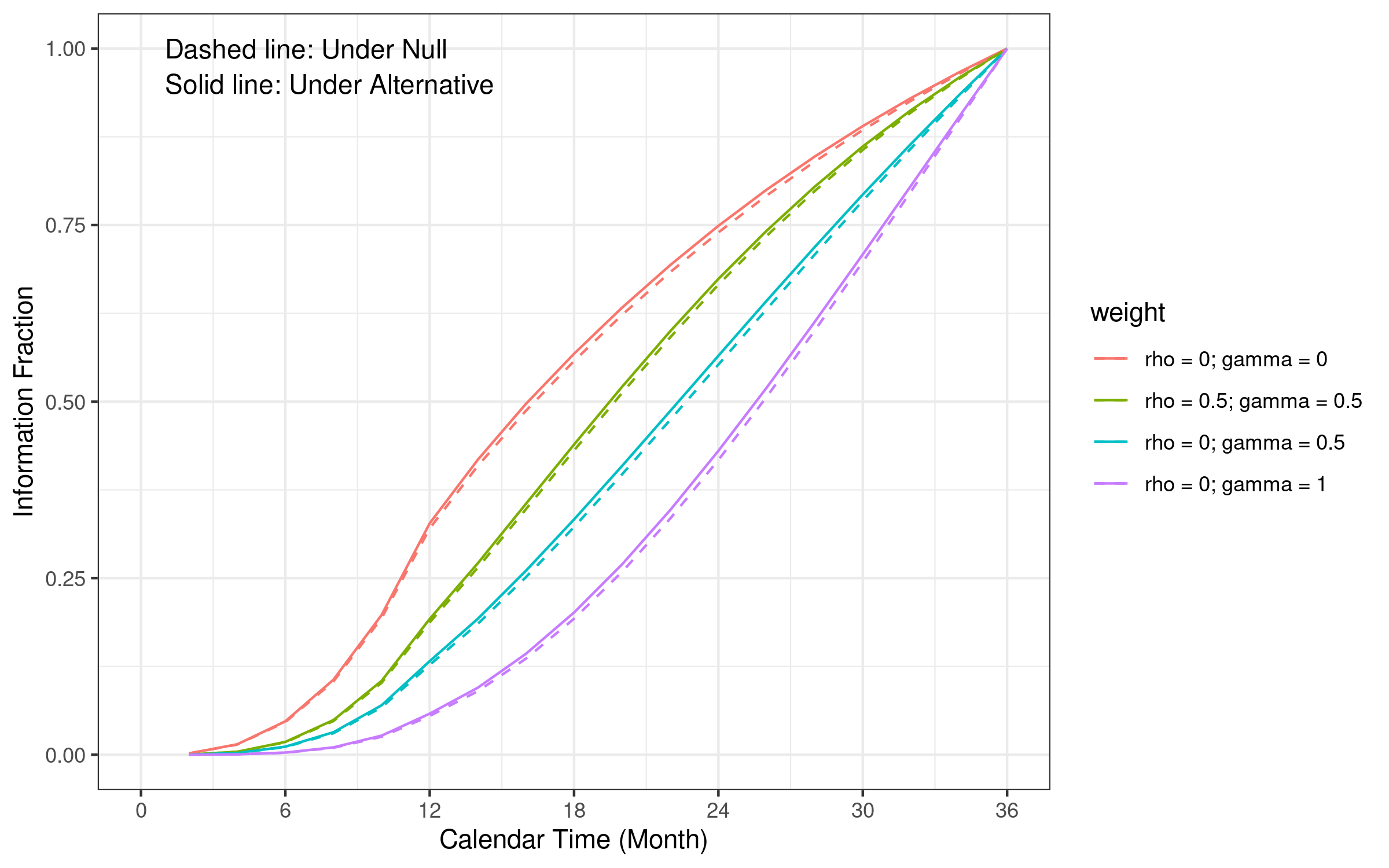
#> # ℹ 2 more variables: info <dbl>, info0 <dbl>9.2 Information fraction
Under the same design assumption, information fraction is different from different weight parameters in WLR.
There are two potential strategies to calculate the information fraction:
- Option 1: Use minimal information fraction of all candidate tests (implemented in gsdmvn).
- Option 2: Use the weighted average of information fraction.
utility <- gsdmvn:::gs_utility_combo(enrollRates, failRates, fh_test = fh_test, ratio = 1)
utility$info_all %>% mutate_if(is.numeric, round, digits = 3)
#>   test Analysis Time   N  Events   AHR  delta sigma2 theta
#> 1    1        1   12 500 107.394 0.842 -0.009  0.054 0.172
#> 2    1        2   24 500 246.283 0.716 -0.041  0.123 0.333
#> 3    1        3   36 500 331.291 0.683 -0.062  0.164 0.381
#> 4    2        1   12 500 107.394 0.781 -0.005  0.007 0.626
#> 5    2        2   24 500 246.283 0.666 -0.024  0.031 0.765
#> 6    2        3   36 500 331.291 0.639 -0.040  0.054 0.732
#> 7    3        1   12 500 107.394 0.790 -0.004  0.006 0.676
#> 8    3        2   24 500 246.283 0.675 -0.019  0.020 0.927
#> 9    3        3   36 500 331.291 0.650 -0.029  0.030 0.973
#>     info  info0
#> 1 26.841 26.899
#> 2 61.352 62.087
#> 3 81.918 83.944
#> 4  3.605  3.624
#> 5 15.371 15.737
#> 6 27.205 28.484
#> 7  2.898  2.910
#> 8 10.155 10.335
#> 9 15.070 15.5269.3 Spending function
-
gsDesign bound can not be directly used for MaxCombo test:
- Multiple test statistics are considered in interim analysis or final analysis.
-
Design example:
- \(\alpha = 0.025\)
- \(\beta = 0.2\)
- \(K=3\) total analysis.
-
test.type=4: A two-sided, asymmetric, beta-spending with non-binding lower bound.
Lan-DeMets spending function to approximate an O’Brien-Fleming bound Gordon Lan and DeMets (1983). (
gsDesign::sfLDOF)\(t\) is information fraction in the formula below.
\[ f(t; \alpha)=2-2\Phi\left(\Phi^{-1}\left(\frac{1-\alpha/2}{t^{\rho/2}}\right)\right) \]
Other spending functions are discussed in the gsDesign technical manual and implemented in
gsDesign::sf*()functions.-
Upper bound:
- Non-binding lower bound: lower bound are all
-Inf.
- Non-binding lower bound: lower bound are all
alpha_spend <- gsDesign::sfLDOF(alpha = 0.025, t = min_info_frac)$spend
alpha_spend
#> [1] 3.300225e-10 2.566068e-03 2.500000e-02- Lower bound:
beta_spend <- gsDesign::sfLDOF(alpha = 0.2, t = min_info_frac)$spend
beta_spend
#> [1] 0.0003269604 0.0846866352 0.2000000000
9.4 Technical details
This section describes the details of calculating the sample size and events required for WLR under group sequential design. It can be skipped for the first read of this training material.
9.5 Upper bound in group sequential design
9.5.1 One test in each interim analysis
- First interim analysis
\[ \alpha_1 = \text{Pr}(Z_1 > b_1 \mid H_0) \]
qnorm(1 - alpha_spend[1])
#> [1] 6.17538- General formula (non-binding futility bound)
\[ \alpha_k = \text{Pr}(\cap_{i=1}^{i=k-1} Z_i < b_i, Z_k > b_k \mid H_0) \]
9.5.2 MaxCombo upper bound
- First interim analysis upper bound
\[ \alpha_1 = \text{Pr}(G_1 > b_1 \mid H_0) = 1 - \text{Pr}(\cap_i Z_{i1} < b_1 \mid H_0) \]
- General formula (non-binding futility bound)
\[ \alpha_k = \text{Pr}(\cap_{i=1}^{i=k-1} G_i < b_i, G_k > b_k \mid H_0) \]
\[ = \text{Pr}(\cap_{i=1}^{i=k-1} G_i < b_i \mid H_0) - \text{Pr}(\cap_{i=1}^{i=k} G_i < b_i \mid H_0) \]
- gsdmvn implementation for MaxCombo test
- Compared with upper bound calculated from gsDesign
x$upper$bound
#> [1] 3.710303 2.511407 1.992970
9.6 Lower bound in group sequential design
9.6.1 One test in each interim analysis
- First interim analysis
\[ \beta_1 = \text{Pr}(Z_1 < a_1 \mid H_1) \]
- General formula
\[ \beta_k = \text{Pr}(\cap_{i=1}^{i=k-1} a_i < Z_i < b_i, Z_k < a_k \mid H_1) \]
9.6.2 MaxCombo lower bound
- First interim analysis upper bound
\[ \beta_1 = \text{Pr}(G_1 < a_1 \mid H_1) = \text{Pr}(\cap_i Z_{i1} < a_1 \mid H_0) \]
- General formula (non-binding futility bound)
\[ \beta_k = \text{Pr}(\cap_{i=1}^{i=k-1} a_i <G_i < b_i, G_k < a_k \mid H_0) \]
- gsdmvn implementation for MaxCombo test
n <- 400
utility <- gsdmvn:::gs_utility_combo(
  enrollRates, failRates, fh_test = fh_test, ratio = 1
)
bound <- gsdmvn:::gs_bound(
  alpha_spend, beta_spend,
  analysis = utility$info$Analysis, # Analysis indicator
  theta = utility$theta * sqrt(n), # Under the alternative hypothesis
  corr = utility$corr # Correlation
)

bound$lower
#> [1] -2.6106678 0.9619422 2.0970774- Compared with lower bound calculated from gsDesign
x$lower$bound
#> [1] -0.2361874  1.1703638  1.9929702
9.7 Sample size calculation
- Sample size and boundaries are set simultaneously using an iterative algorithm.
9.7.1 Initiate the calculation from lower bound derived at \(N = 400\)
bound
#>      upper      lower
#> 1 6.175397 -2.6106678
#> 2 2.798651  0.9619422
#> 3 2.097077 2.0970774gs_design_combo(
enrollRates,
failRates,
fh_test,
alpha = 0.025,
beta = 0.2,
ratio = 1,
binding = FALSE,
upar = bound$upper,
lpar = bound$lower,
) %>% mutate_if(is.numeric, round, digits = 2)
#> Analysis Bound Time N Events Z Probability
#> 1 1 Upper 12 324.92 69.79 6.18 0.00
#> 3 2 Upper 24 324.92 160.05 2.80 0.24
#> 5 3 Upper 36 324.92 215.29 2.10 0.80
#> 2 1 Lower 12 324.92 69.79 -2.61 0.00
#> 4 2 Lower 24 324.92 160.05 0.96 0.13
#> 6 3 Lower 36 324.92 215.29 2.10 0.20
#> Probability_Null
#> 1 0.00
#> 3 0.00
#> 5 0.03
#> 2 NA
#> 4 NA
#> 6 NA9.7.2 Update bound based on newly calculated sample size
n <- 355
utility <- gsdmvn:::gs_utility_combo(enrollRates, failRates, fh_test = fh_test, ratio = 1)
bound <- gsdmvn:::gs_bound(alpha_spend, beta_spend,
  analysis = utility$info$Analysis, # Analysis indicator
  theta = utility$theta * sqrt(n), # Under the alternative hypothesis
  corr = utility$corr # Correlation
)

bound
#>      upper      lower
#> 1 6.175397 -2.6568642
#> 2 2.798651  0.8266125
#> 3 2.097372 2.0973716- Repeat the procedure above until the sample size and lower bound converge.