6 Weighted logrank test
In this chapter, we start to discuss group sequential design for weighted logrank test.
6.1 Assumptions
For a group sequential design, we assume there are total \(K\) analyses in a trial. The calendar time of the analyses are \(t_k, k =1,\dots, K\).
We define the test statistic at analysis \(k=1,2,\dots,K\) as
\[ Z_k = \frac{\widehat{\Delta}_k}{\sigma(\widehat{\Delta}_k)} \]
where \(\widehat{\Delta}_k\) is a statistics to characterize group difference and \(\sigma(\widehat{\Delta}_k)\) is the standard deviation of \(\widehat{\Delta}_k\).
6.1.1 Asymptotic normality
In group sequential design, we consider the test statistics are asymptotically normal.
- Under the null hypothesis
\[ Z_k \sim \mathcal{N}(0,1) \]
- Under a (local) alternative hypothesis
\[ Z_k \sim \mathcal{N}(\Delta_k I_k^{1/2}, 1), \]
where \(I_k\) is the Fisher information \(I_k \approx 1/{\sigma^2(\widehat{\Delta}_k)}\)
Then we can define the effect size as
\[ \theta = \Delta_k / \sigma_k = \Delta_k I_k^{1/2}$ with $\sigma_k = \sigma(\widehat{\Delta}_k) \].
So, it is equivalent to claim:
\[ Z_k \sim \mathcal{N}(\theta_k, 1) \]
6.1.2 Independent increments process
For group sequential design, we need to demonstrate the test statistics \(Z = (Z_1, \dots, Z_K)\) is an independent increments process. The property for WLR has been proved by Scharfstein, Tsiatis, and Robins (1997) as a corollary of martingale representation.
Under the null \(Z ~ \sim MVN(0,\Sigma)\)
Under a local alternative \(Z ~ \sim MVN(\theta, \Sigma)\)
Here, \(\Sigma={\Sigma_{ij}}\) is a correlation matrix with
\[ \Sigma_{ij} = \min(I_i, I_j) / \max(I_i, I_j) \approx \min(\sigma_i, \sigma_j) / \max(\sigma_i, \sigma_j) \]
6.2 Type I error, \(\alpha\)-spending function, and group sequential design boundary
- Define test boundary for each interim analysis
- \(\alpha\)-spending function Lan and DeMets (1983)
- Bounds \(-\infty \le a_k \le b_k \le \infty\) for \(k=1,\dots,K\)
- non-binding futility bound \(a_k = -\infty\) for all \(k\)
- Upper boundary crossing probabilities
- \(u_k = \text{Pr}(\{Z_k \ge b_k\} \cap_{j=1}^{k-1} \{a_j \le Z_j < b_j\})\)
- Lower boundary crossing probabilities
- \(l_k = \text{Pr}(\{Z_k < a_k\} \cap_{j=1}^{k-1} \{a_j \le Z_j < b_j\})\)
- Under the null hypothesis, the probability to reject the null hypothesis.
- \(\alpha = \sum_{k=1}^{K} u_k = \sum_{k=1}^{K} \text{Pr}(\{Z_k \ge b_k\} \cap_{j=1}^{k-1} \{a_j \le Z_j \le b_j\} \mid H_0)\)
- With a spending function family \(f(t,\gamma)\),
-
gsDesign::sfLDOF()(O’Brien-Fleming bound approximation) or other functions starts withsfin gsDesign
For simplicity, we directly use gsDesign boundary for this chapter. It will inflate Type I Error for WLR tests. We will discuss how to fix the issue in the next chapter.
- Lower bound
x$lower$bound
#> [1] -0.6945842 1.0023997 1.9929702- Upper bound
x$upper$bound
#> [1] 3.710303 2.511407 1.992970
6.3 Power
Given the lower and upper bound of a group sequential design, we can calculate the overall power of the design.
- Power: under a (local) alternative hypothesis, the probability to reject the null hypothesis.
\[ 1 - \beta =\sum_{k=1}^{K} u_k = \sum_{k=1}^{K} \text{Pr}(\{Z_k \ge b_k\} \cap_{j=1}^{k-1} \{a_j \le Z_j \le b_j\} \mid H_1) \]
If there is no lower bound, the formula can be simplified as
\[ \beta = \text{Pr}(\cap_{j=1}^{K} \{Z_j \le b_j\} \mid H_1) \]
We can calculate the sample size required for a group sequential design by solving the power equation with a given lower and upper bound and power, type I error and power.
As a note, we can calculate futility probability similarly:
\[ \sum_{k=1}^{K} l_k = \sum_{k=1}^{K} \text{Pr}(\{Z_k < a_k\} \cap_{j=1}^{k-1} \{a_j \le Z_j \le b_j\}\mid H_1) \]
6.4 Weighted logrank test
Similar to the fixed design, we can define the test statistics for weighted logrank test using the counting process formula as
\[ Z_k=\sqrt{\frac{n_{0}+n_{1}}{n_{0}n_{1}}}\int_{0}^{t_k}w(t)\frac{\overline{Y}_{0}(t)\overline{Y}_{1}(t)}{\overline{Y}_{0}(t)+\overline{Y}_{0}(t)}\left\{ \frac{d\overline{N}_{1}(t)}{\overline{Y}_{1}(t)}-\frac{d\overline{N}_{0}(t)}{\overline{Y}_{0}(t)}\right\} \]
Here \(n_i\) are the number of subjects in group \(i\). \(\overline{Y}_{i}(t)\) are the number of subjects in group \(i\) at risk at time \(t\). \(\overline{N}_{i}(t)\) are the number of events in group \(i\) up to and including time \(t\).
Note, the only difference is that the test statistics fixed analysis up to \(t_k\) at \(k\)th interim analysis
For simplicity, we illustrate the sample size and power calculation based on the boundary from the logrank test. The same boundary for different types of analysis for a fair comparison. However, different WLR can have different information fraction for the same interim analysis time. Further discussion of the spending function based on actual information fraction will be provided later.
6.5 Example scenario
We considered an example scenario that is similar to the fixed design. The key difference is that we considered 2 interim analysis at 12 and 24 months before the final analysis at 36 months.
# Randomization Ratio is 1:1
ratio <- 1

# Type I error (one-sided)
alpha <- 0.025

# Power (1 - beta)
beta <- 0.2
power <- 1 - beta

# Interim Analysis Time
analysisTimes <- c(12, 24, 36)
6.6 Sample size under logrank test or \(FH(0, 0)\)
In gsdmvn, the sample size can be calculated using gsdmvn::gs_design_wlr() for the WLR test. For comparison purposes, we also provided the sample size calculation using gsdmvn::gs_design_ahr() for the logrank test. In each calculation, we compare the analytical results with the simulation results with 10,000 replications.
We described the theoretical details for sample size calculation in the technical details section.
- AHR with logrank test
gsdmvn::gs_design_ahr(
  enrollRates = enrollRates, failRates = failRates,
  ratio = ratio, alpha = alpha, beta = beta,
  upar = x$upper$bound,
  lpar = x$lower$bound,
  analysisTimes = analysisTimes
)$bounds %>%
  mutate_if(is.numeric, round, digits = 2) %>%
  select(Analysis, Bound, Time, N, Events, AHR, Probability) %>%
  tidyr::pivot_wider(names_from = Bound, values_from = Probability)
#> # A tibble: 3 × 7
#>   Analysis  Time     N Events   AHR Upper Lower
#>      <dbl> <dbl> <dbl>  <dbl> <dbl> <dbl> <dbl>
#> 1        1    12  386.   82.9  0.84  0     0.07
#> 2        2    24  386.  190.   0.71  0.41  0.13
#> 3 3 36 386. 256. 0.68 0.8 0.2- Simulation results based on 10,000 replications.
#>      n  t events  ahr lower upper
#> 10 386 12  82.77 0.87  0.07  0.00
#> 11 386 24 190.05 0.72  0.14  0.41
#> 12 386 36 255.61 0.69 0.20 0.80- \(FH(0,0)\)
gsdmvn::gs_design_wlr(
  enrollRates = enrollRates, failRates = failRates,
  weight = function(x, arm0, arm1) {
    gsdmvn::wlr_weight_fh(x, arm0, arm1, rho = 0, gamma = 0)
  },
  ratio = ratio, alpha = alpha, beta = beta,
  upar = x$upper$bound,
  lpar = x$lower$bound,
  analysisTimes = c(12, 24, 36)
)$bounds %>%
  mutate_if(is.numeric, round, digits = 2) %>%
  select(Analysis, Bound, Time, N, Events, AHR, Probability) %>%
  tidyr::pivot_wider(names_from = Bound, values_from = Probability)
#> # A tibble: 3 × 7
#>   Analysis  Time     N Events   AHR Upper Lower
#>      <dbl> <dbl> <dbl>  <dbl> <dbl> <dbl> <dbl>
#> 1        1    12  383.   82.3  0.84  0     0.07
#> 2        2    24  383.  189.   0.72  0.41  0.14
#> 3 3 36 383. 254. 0.68 0.8 0.2- Simulation results based on 10,000 replications.
#>     n  t events  ahr lower upper
#> 4 384 12  82.36 0.86  0.07  0.00
#> 5 384 24 189.05 0.72  0.14  0.41
#> 6 384 36 254.30 0.69  0.20  0.80
6.7 Sample size under modestly WLR cut at 4 months
- Modestly WLR: \(S^{-1}(t\land\tau_m)\) Magirr and Burman (2019)
gsdmvn::gs_design_wlr(
  enrollRates = enrollRates, failRates = failRates,
  weight = function(x, arm0, arm1) {
    gsdmvn::wlr_weight_fh(x, arm0, arm1, rho = -1, gamma = 0, tau = 4)
  },
  ratio = ratio, alpha = alpha, beta = beta,
  upar = x$upper$bound,
  lpar = x$lower$bound,
  analysisTimes = analysisTimes
)$bounds %>%
  mutate_if(is.numeric, round, digits = 2)
#> # A tibble: 6 × 11
#>   Analysis Bound  Time     N Events     Z Probability   AHR theta
#>      <dbl> <chr> <dbl> <dbl>  <dbl> <dbl>       <dbl> <dbl> <dbl>
#> 1        1 Upper    12  365.   78.5  3.71        0     0.83  0.16
#> 2        2 Upper    24  365.  180.   2.51        0.41  0.71  0.29
#> 3        3 Upper    36  365.  242.   1.99        0.8   0.68  0.33
#> 4        1 Lower    12  365.   78.5 -0.69        0.07  0.83  0.16
#> 5        2 Lower    24  365.  180.   1           0.13  0.71  0.29
#> 6        3 Lower    36  365.  242.   1.99        0.2   0.68  0.33
#> # ℹ 2 more variables: info <dbl>, info0 <dbl>
6.8 Sample size under \(FH(0, 1)\)
gsdmvn::gs_design_wlr(
  enrollRates = enrollRates, failRates = failRates,
  weight = function(x, arm0, arm1) {
    gsdmvn::wlr_weight_fh(x, arm0, arm1, rho = 0, gamma = 1)
  },
  ratio = ratio, alpha = alpha, beta = beta,
  upar = x$upper$bound,
  lpar = x$lower$bound,
  analysisTimes = analysisTimes
)$bounds %>%
  mutate_if(is.numeric, round, digits = 2) %>%
  select(Analysis, Bound, Time, N, Events, AHR, Probability) %>%
  tidyr::pivot_wider(names_from = Bound, values_from = Probability)
#> # A tibble: 3 × 7
#>   Analysis  Time     N Events   AHR Upper Lower
#>      <dbl> <dbl> <dbl>  <dbl> <dbl> <dbl> <dbl>
#> 1        1    12  316.   68.0  0.73  0     0.04
#> 2        2    24  316.  156.   0.64  0.45  0.11
#> 3 3 36 316. 210. 0.62 0.8 0.2- Simulation results based on 10,000 replications.
#>      n  t events  ahr lower upper
#> 16 317 12  68.01 0.76  0.04  0.00
#> 17 317 24 156.13 0.65  0.12  0.45
#> 18 317 36 210.06 0.63  0.21  0.79
6.9 Sample size under \(FH(0, 0.5)\)
gsdmvn::gs_design_wlr(
  enrollRates = enrollRates, failRates = failRates,
  weight = function(x, arm0, arm1) {
    gsdmvn::wlr_weight_fh(x, arm0, arm1, rho = 0, gamma = 0.5)
  },
  ratio = ratio, alpha = alpha, beta = beta,
  upar = x$upper$bound,
  lpar = x$lower$bound,
  analysisTimes = analysisTimes
)$bounds %>%
  mutate_if(is.numeric, round, digits = 2) %>%
  select(Analysis, Bound, Time, N, Events, AHR, Probability) %>%
  tidyr::pivot_wider(names_from = Bound, values_from = Probability)
#> # A tibble: 3 × 7
#>   Analysis  Time     N Events   AHR Upper Lower
#>      <dbl> <dbl> <dbl>  <dbl> <dbl> <dbl> <dbl>
#> 1        1    12  314.   67.4  0.78  0     0.05
#> 2        2    24  314.  155.   0.67  0.44  0.12
#> 3 3 36 314. 208. 0.64 0.8 0.2- Simulation results based on 10,000 replications.
#>      n  t events  ahr lower upper
#> 22 314 12  67.21 0.81  0.05  0.00
#> 23 314 24 154.43 0.67  0.12  0.44
#> 24 314 36 207.92 0.65  0.21  0.79
6.10 Sample size under \(FH(0.5, 0.5)\)
gsdmvn::gs_design_wlr(
  enrollRates = enrollRates, failRates = failRates,
  weight = function(x, arm0, arm1) {
    gsdmvn::wlr_weight_fh(x, arm0, arm1, rho = 0.5, gamma = 0.5)
  },
  ratio = ratio, alpha = alpha, beta = beta,
  upar = x$upper$bound,
  lpar = x$lower$bound,
  analysisTimes = analysisTimes
)$bounds %>%
  mutate_if(is.numeric, round, digits = 2) %>%
  select(Analysis, Bound, Time, N, Events, AHR, Probability) %>%
  tidyr::pivot_wider(names_from = Bound, values_from = Probability)
#> # A tibble: 3 × 7
#>   Analysis  Time     N Events   AHR Upper Lower
#>      <dbl> <dbl> <dbl>  <dbl> <dbl> <dbl> <dbl>
#> 1        1    12  317.   68.0  0.79  0     0.05
#> 2        2    24  317.  156    0.68  0.43  0.12
#> 3 3 36 317. 210. 0.65 0.8 0.2- Simulation results based on 10,000 replications.
#>      n  t events  ahr lower upper
#> 28 317 12  67.87 0.81  0.06  0.00
#> 29 317 24 155.86 0.68  0.12  0.43
#> 30 317 36 209.82 0.66  0.20  0.80
6.11 Average hazard ratio comparison
The average hazard ratio depends on the weight used in the WLR. We illustrate the difference in the figure below.
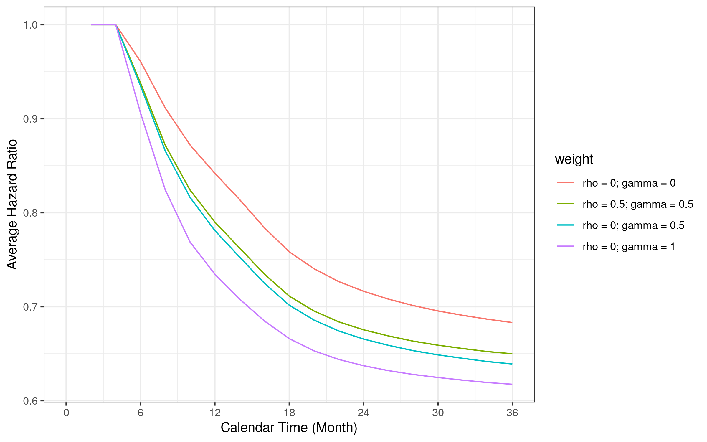
Note that the average hazard ratio is weighted by corresponding weighted logrank weights.
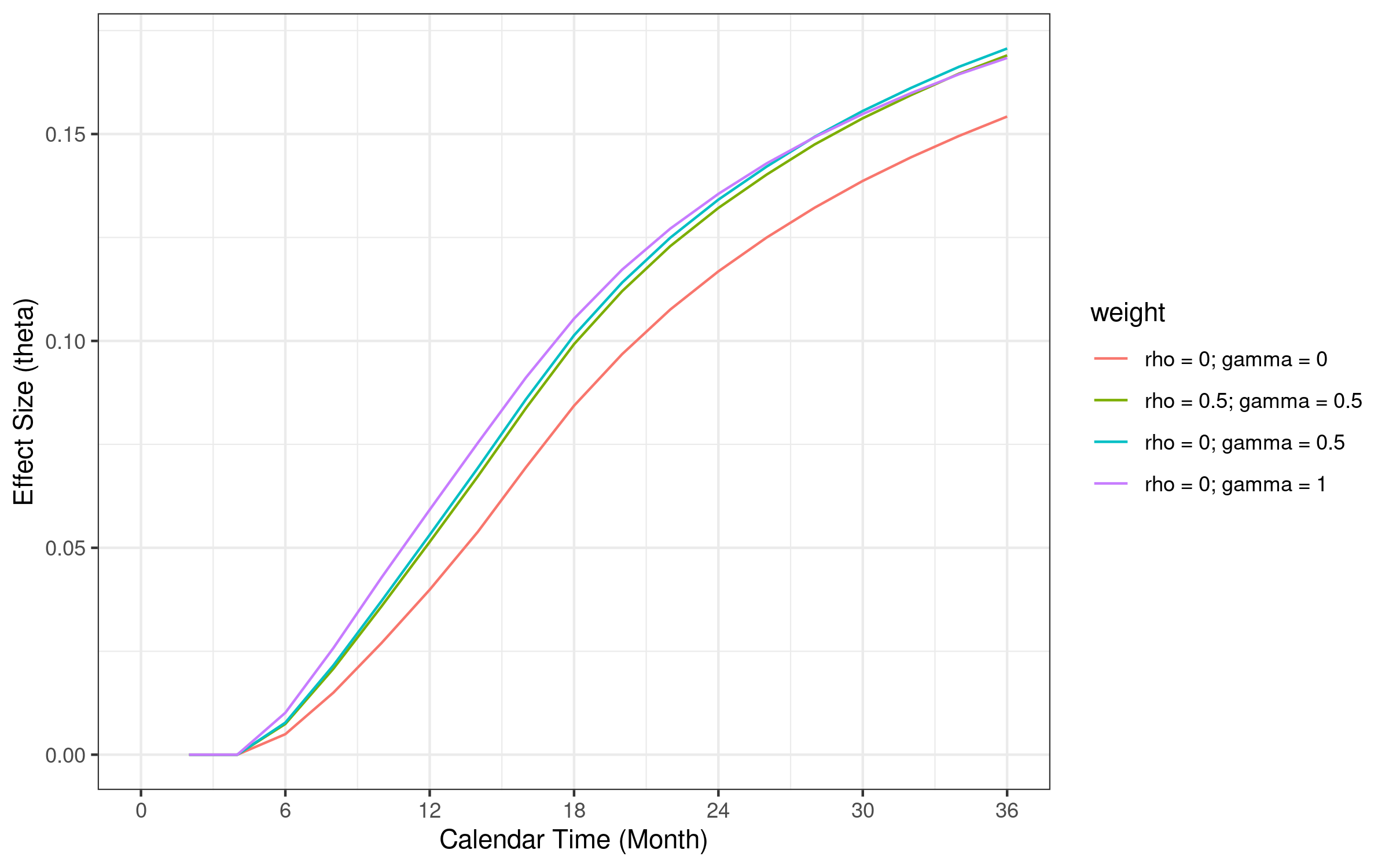
6.12 Standardized effect size comparison
Standardized effect size of \(FH(0, 0.5)\) is larger than other weight function at month 36. The reason \(FH(0.5, 0.5)\) provides slightly smaller sample size compared with \(FH(0, 1)\) and \(FH(0, 0.5)\) is mainly due to smaller weight when variance becomes larger than \(FH(0, 1)\) with later events.
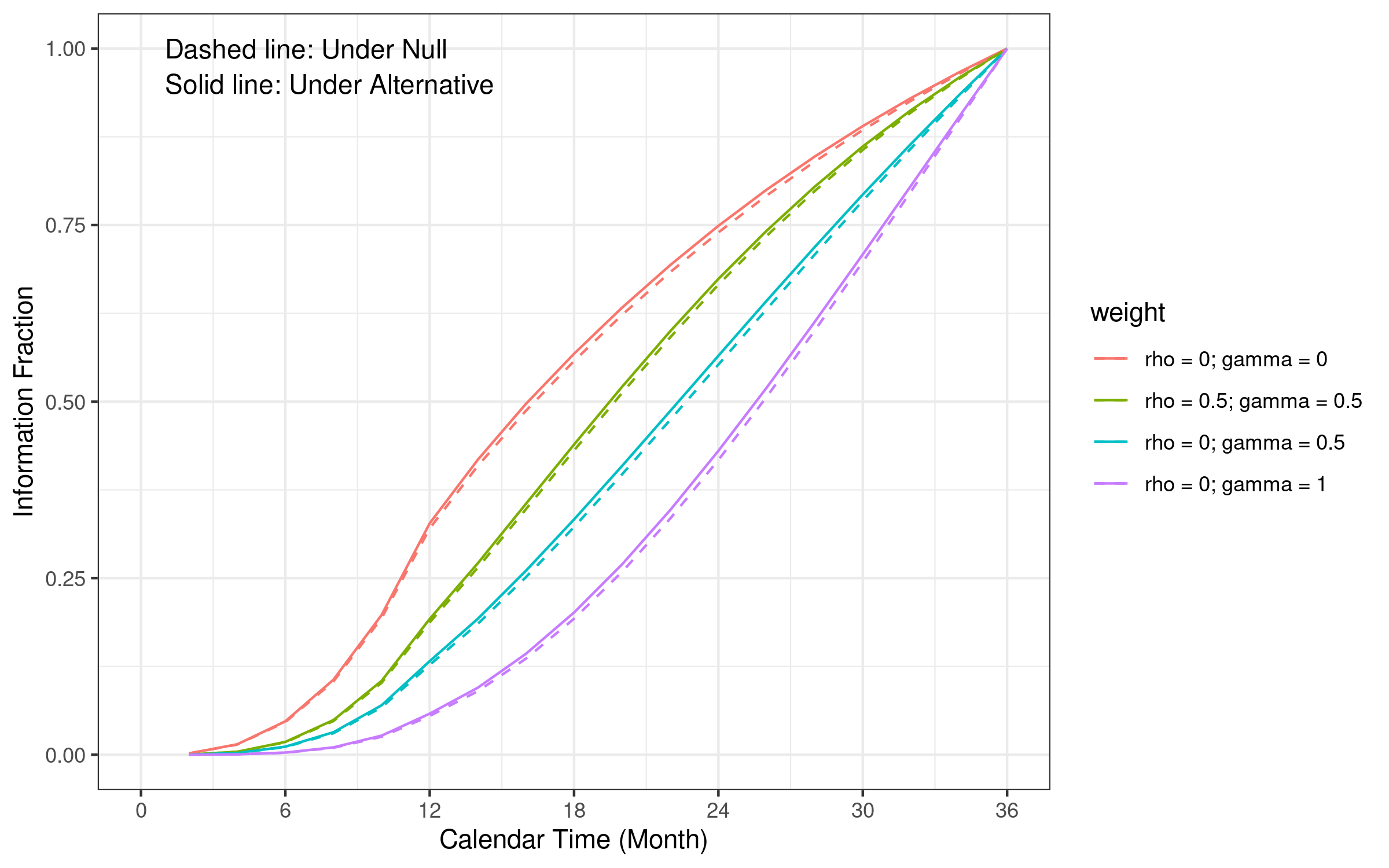
6.13 Information fraction comparison
The logrank test information fraction curve is close to a linear function of time (the boundary calculation approach we used). Other WLR test information fraction curves are convex functions. Information fraction under the null hypothesis is smaller than information fraction under alternative at the same time.
6.14 Technical details
This section describes the details of calculating the sample size and events required for WLR under group sequential design. It can be skipped for the first read of this training material.
We illustrate the idea using \(FH(0, 1)\).
weight <- function(x, arm0, arm1) {
  gsdmvn::wlr_weight_fh(x, arm0, arm1, rho = 0, gamma = 1)
}
# Define study design object in each arm
gs_arm <- gsdmvn:::gs_create_arm(
enrollRates, failRates,
ratio = 1, # Randomization ratio
total_time = 36 # Total study duration
)
arm0 <- gs_arm[["arm0"]]
arm1 <- gs_arm[["arm1"]]The calculation of power is essentially the multiple integration of multivariate normal distribution, and we implement it into a function gs_power() where mvtnorm::pmvnorm() is used to take care of the multiple integration.
#' Power and futility of group sequential design
#'
#' @param z Numerical vector of Z statistics
#' @param corr Correlation matrix of Z statistics
#' @param futility_bound Numerical vector of futility bound.
#'                       -Inf indicates non-binding futility bound.
#' @param efficacy_bound Numerical vector of efficacy bound.
#'                       Inf indicates no early stop to declare superiority.
gs_power <- function(z, corr, futility_bound, efficacy_bound) {
  p <- c()
  p[1] <- 1 - pnorm(efficacy_bound[1], mean = z[1], sd = 1)

  for (k in 2:length(z)) {
    lower_k <- c(futility_bound[1:(k - 1)], efficacy_bound[k])
    upper_k <- c(efficacy_bound[1:(k - 1)], Inf)
    p[k] <- mvtnorm::pmvnorm(
      lower = lower_k, upper = upper_k,
      mean = z[1:k], corr = corr[1:k, 1:k]
    )
  }

  p
}
To utilize gs_power(), four important blocks are required.
- The expectation mean of Z statistics. To derive it, one needs \(\Delta_k\), \(\sigma_k^{2}\) and sample size ratio at each interim analysis.
- The correlation matrix of Z statistics (denoted as \(\Sigma\)).
- The numerical vector of futility bound for multiple integration.
- The numerical vector of efficacy bound for multiple integration.
First, we calculate
\[ \Delta_k = \int_{0}^{t_k}w(s)\frac{p_{0}\pi_{0}(s)p_{1}\pi_{1}(s)}{\pi(s)}\{\lambda_{1}(s)-\lambda_{0}(s)\}ds, \]
where \(p_0 = n_0/(n_0 + n_1), p_1 = n_1/(n_0 + n_1)\) are the randomization ratio of the control and treatment arm, respectively. \(\pi_0(t) = E(N_0(t)), \pi_1(t) = E(N_1(t))\) are the expected number of failures of the control and treatment arm, respectively. \(\pi(t) = p_0 \pi_0(t) + p_1 \pi_1(t)\) is the probability of events. \(\lambda_0(t), \lambda_1(t)\) are hazard functions. The detailed calculation of \(\Delta_k\) is implemented in gsdmvn:::gs_delta_wlr():
Second, we calculate
\[ \sigma_k^{2}=\int_{0}^{t_k}w(s)^{2}\frac{p_{0}\pi_{0}(s)p_{1}\pi_{1}(s)}{\pi(s)^{2}}dv(s), \]
where \(v(t)= p_0 E(Y_0(t)) + p_1 E(Y_1(t))\) is the probability of people at risk. The detailed calculation of \(\sigma_k^{2}\) is implemented in gsdmvn:::gs_sigma2_wlr():
Third, the sample size ratio at each interim analysis can be calculated by
After getting \(\Delta_k\), \(\sigma_k^{2}\), and the sample size ratio, one can calculate the expectation mean of Z statistics as
Then, we calculate the correlation matrix \(\Sigma\) as
Finally, for numerical vector of futility and bound, they are simply
x$lower$bound
#> [1] -0.6945842  1.0023997  1.9929702
x$upper$bound
#> [1] 3.710303 2.511407 1.992970
6.14.1 Power and sample size calculation
- Power
With all blocks prepared, one can calculate the power
\[ 1 -\beta = \sum_{k=1}^{K} u_k = \sum_{k=1}^{K} \text{Pr}(\{Z_k \ge b_k\} \cap_{j=1}^{k-1} \{a_j \le Z_j \le b_j\}) \]
by
- Type I error
One can also calculate the type I error by
- Futility probability
Similarly, we can calculate the futility probability
\[ \sum_{k=1}^{K} l_k = \sum_{k=1}^{K} \text{Pr}(\{Z_k < a_k\} \cap_{j=1}^{k-1} \{a_j \le Z_j \le b_j\}) \]
by
#' @rdname power_futility
gs_futility <- function(z, corr, futility_bound, efficacy_bound) {
  p <- c()
  p[1] <- pnorm(futility_bound[1], mean = z[1], sd = 1)

  for (k in 2:length(z)) {
    lower_k <- c(futility_bound[1:(k - 1)], -Inf)
    upper_k <- c(efficacy_bound[1:(k - 1)], futility_bound[k])
    p[k] <- mvtnorm::pmvnorm(
      lower = lower_k, upper = upper_k,
      mean = z[1:k], corr = corr[1:k, 1:k]
    )
  }

  p
}- Sample size
In addition to power and futility probability, one can also calculate the sample size by
n_subject <- n * ratio / sum(ratio)
n_subject * gs_n_ratio
#> [1] 316.4479 316.4479 316.4479- Number of events
With the sample size available, one can calculate the number of events by
n0 <- n1 <- n_subject / 2
gsdmvn:::prob_event.arm(arm0, tmax = analysisTimes) * n0 +
  gsdmvn:::prob_event.arm(arm1, tmax = analysisTimes) * n1
#> [1] 67.96939 155.87175 209.67266- Average hazard ratio
The function below implements the connection between \(\Delta\) and average hazard ratio using Taylor series expansion.
- The
infocolumn is \(\sigma^2_k\) times \(N\)
n_subject * sigma2
#> [1] 0.4466842 3.3047797 7.6793673- The
info0column is \(\sigma^2_k\) times \(N\) under the null where we both usearm0for calculation in active and control group.
6.14.2 Cross comparison with gs_design_wlr()
gsdmvn::gs_design_wlr(
  enrollRates = enrollRates, failRates = failRates,
  weight = function(x, arm0, arm1) {
    gsdmvn::wlr_weight_fh(x, arm0, arm1, rho = 0, gamma = 1)
  },
  ratio = ratio, alpha = alpha, beta = beta,
  upar = x$upper$bound,
  lpar = x$lower$bound,
  analysisTimes = analysisTimes
)$bounds %>%
  mutate_if(is.numeric, round, digits = 2)
#> # A tibble: 6 × 11
#>   Analysis Bound  Time     N Events     Z Probability   AHR theta
#>      <dbl> <chr> <dbl> <dbl>  <dbl> <dbl>       <dbl> <dbl> <dbl>
#> 1        1 Upper    12  316.   68.0  3.71        0     0.73  1.58
#> 2        2 Upper    24  316.  156.   2.51        0.45  0.64  1.33
#> 3        3 Upper    36  316.  210.   1.99        0.8   0.62  1.08
#> 4        1 Lower    12  316.   68.0 -0.69        0.04  0.73  1.58
#> 5        2 Lower    24  316.  156.   1           0.11  0.64  1.33
#> 6        3 Lower    36  316.  210.   1.99        0.2   0.62  1.08
#> # ℹ 2 more variables: info <dbl>, info0 <dbl>
6.14.3 Illustration of gs_info_wlr()
The necessary information has also been summarized in a data frame using gsdmvn::gs_info_wlr().
gs_info <- gsdmvn::gs_info_wlr(
  enrollRates, failRates, ratio,
  analysisTimes = analysisTimes,
  weight = weight
)

gs_info %>% mutate_if(is.numeric, round, digits = 2)
#>   Analysis Time   N Events  AHR delta sigma2 theta  info info0
#> 1        1   12 500 107.39 0.73  0.00   0.00  1.58  0.71  0.71
#> 2        2   24 500 246.28 0.64 -0.01   0.01  1.33  5.22  5.41
#> 3 3 36 500 331.29 0.62 -0.03 0.02 1.08 12.13 12.96-
Nis based on the information inenrollRates
N <- sum(enrollRates$rate * enrollRates$duration)
N
#> [1] 500-
Eventsis the probability of events times \(N\)
n0 <- n1 <- N / 2
gsdmvn:::prob_event.arm(arm0, tmax = analysisTimes) * n0 +
  gsdmvn:::prob_event.arm(arm1, tmax = analysisTimes) * n1
#> [1] 107.3943 246.2834 331.2909-
AHRis the average hazard ratio
-
delta,sigma2, andthetaare defined as above
delta / sigma2
#> [1] 1.577775 1.326384 1.081194- The
infocolumn is \(\sigma^2_k\) times \(N\)
N * sigma2
#> [1] 0.7057784 5.2216800 12.1336979- The
info0column is \(\sigma^2_k\) times \(N\) under the null.