8 Group sequential design boundary with weighted logrank test

8.1 Group sequential design boundary calculation strategy

In the last chapter, we pre-specified boundary derived from gsDesign. Therefore, the Type I error may be inflated because the information fraction is different for different WLR.

In this chapter, we calculate boundaries based on the error spending approach following Gordon Lan and DeMets (1983).

The spending function has been implemented in gsDesign.

gsDesign::sfLDOF() (O’Brien-Fleming bound approximation) or other functions starting with sf in gsDesign
The boundary family approach. Pocock (1977), O’Brien and Fleming (1979), Wang and Tsiatis (1987)

There are other ways to derive boundaries but will not be covered:

Conditional power (Lachin 2005)

8.2 Types of error probability

There are 6 different types of error probability that have been implemented in gsdmvn. In this training material, we focus on test.type = 4.

test.type argument in gsDesign
Upper bound:
- \(\alpha_k(0) = \text{Pr}(\cap_{i=1}^{i=k-1} a_i < Z_i < b_i, Z_k > b_k \mid H_0)\)
- \(\alpha_k^{+}(0) = \text{Pr}(\cap_{i=1}^{i=k-1} a_i < Z_i < b_i, Z_k > b_k \mid H_0)\) (ignore lower bound)

Lower bound:

\(\beta_k(0) = \text{Pr}(\cap_{i=1}^{i=k-1} a_i < Z_i < b_i, Z_k < a_k \mid H_0)\) (under null)
\(\beta_k(\delta) = \text{Pr}(\cap_{i=1}^{i=k-1} a_i < Z_i < b_i, Z_k < a_k \mid H_1)\) (under alternative)

`test.type`	Upper bound	Lower bound
1	\(\alpha_k^{+}(0)\)	None
2	\(\alpha(0)\)	\(\beta_k(0)\)
3	\(\alpha_k(0)\)	\(\beta_k(\delta)\)
4	\(\alpha_k^{+}(0)\)	\(\beta_k(\delta)\)
5	\(\alpha(0)\)	\(\beta_k(0)\)
6	\(\alpha^{+}(0)\)	\(\beta_k(0)\)

test.type = 1, 2, 5, 6: sample size boundaries can be computed in a single step.
test.type = 3 and test.type = 4: sample size and boundaries are set simultaneously using an iterative algorithm.
This section and last section focus on test.type = 4.

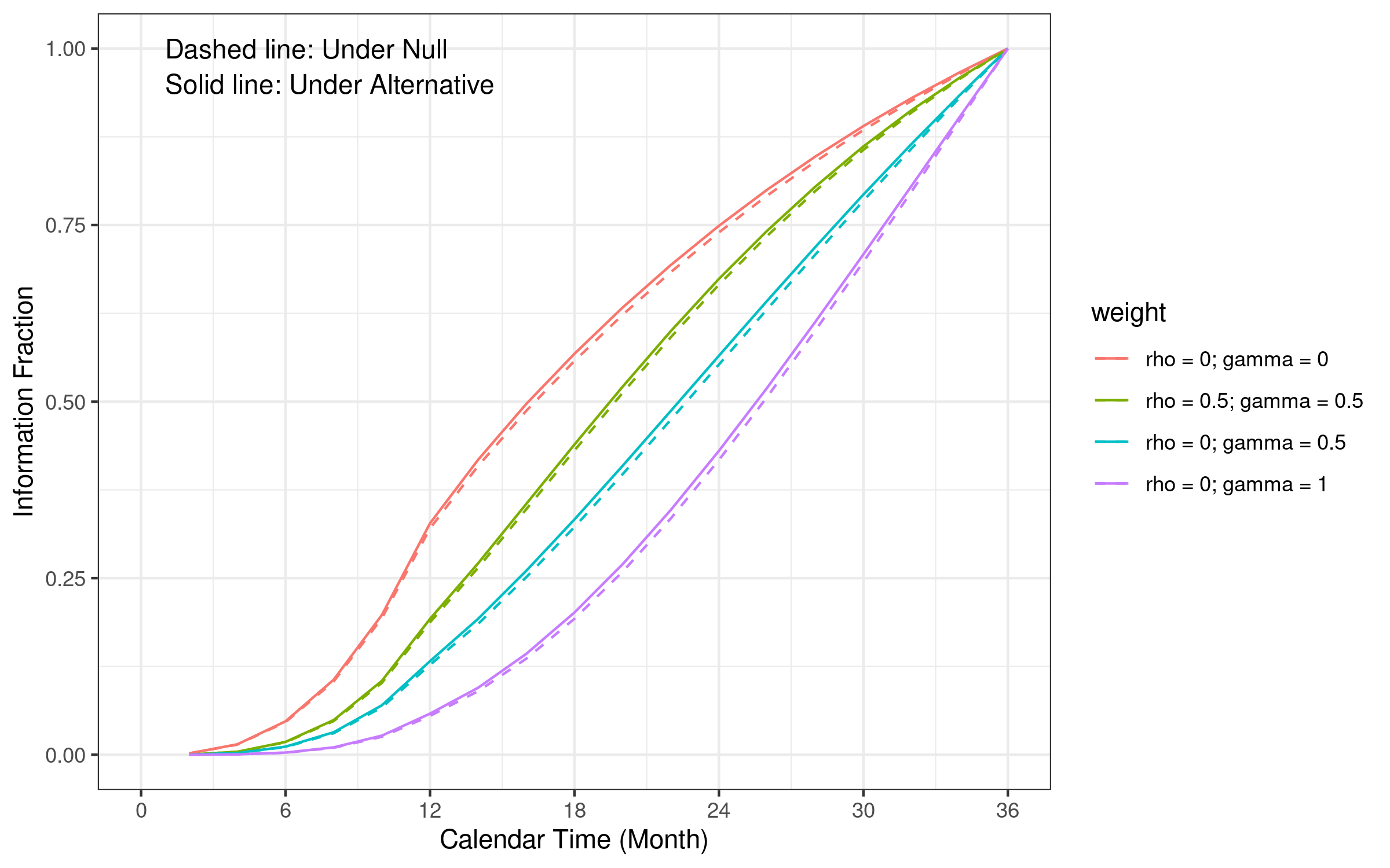
8.3 Information fraction

Under the same design assumption, information fraction is different from different weight parameters in WLR.

We continue using the same example scenario in the last chapter.

8.4 Spending function based on information fraction

The spending function is based on information fraction. We considered the Lan-DeMets spending function to approximate an O’Brien-Fleming bound Gordon Lan and DeMets (1983). (gsDesign::sfLDOF()).

Here, \(t\) is information fraction in the formula below.

\[f(t; \alpha)=2-2\Phi\left(\Phi^{-1}\left(\frac{1-\alpha/2}{t^{\rho/2}}\right)\right)\]

8.4.1 Spending function in `gsDesign`

After the spending function is selected, we can calculate the lower and upper bound of a group sequential design.

In test type 4, the lower bound is non-binding. So we set lower bound are all -Inf when we calculate the probability to cross upper bound.

We first use the alpha spending function to determine the upper bound of a group sequential design

Let \((a_k, b_k), k=1,\dots, K\) denotes the lower and upper bound.

For gsDesign with logrank test, we considered equal increments of information fraction at t = 1:3 / 3 is.

The upper bound and lower bound based on the Lan-DeMets spending function can be calculated using gsDesign::sfLDOF().

Upper bound:

alpha_spend <- gsDesign::sfLDOF(alpha = 0.025, t = 1:3 / 3)$spend
alpha_spend

#> [1] 0.0001035057 0.0060483891 0.0250000000

Lower bound:

beta_spend <- gsDesign::sfLDOF(alpha = 0.2, t = 1:3 / 3)$spend
beta_spend

#> [1] 0.02643829 0.11651432 0.20000000

We considered different WLR tests with weight functions: \(FH(0, 0)\), \(FH(0.5, 0.5)\), \(FH(0, 0.5)\), \(FH(0, 1)\)

weight_fun <- list(
  function(x, arm0, arm1) {
    gsdmvn::wlr_weight_fh(x, arm0, arm1, rho = 0, gamma = 0)
  },
  function(x, arm0, arm1) {
    gsdmvn::wlr_weight_fh(x, arm0, arm1, rho = 0.5, gamma = 0.5)
  },
  function(x, arm0, arm1) {
    gsdmvn::wlr_weight_fh(x, arm0, arm1, rho = 0, gamma = 0.5)
  },
  function(x, arm0, arm1) {
    gsdmvn::wlr_weight_fh(x, arm0, arm1, rho = 0, gamma = 1)
  }
)

# Weight name
weight_name <- data.frame(rho = c(0, 0.5, 0, 0), gamma = c(0, 0.5, 0.5, 1))
weight_name <- with(weight_name, paste0("rho = ", rho, "; gamma = ", gamma))

For test type 4, the alpha and beta is defined as below.

\(\alpha_k^{+}(0) = \text{Pr}(\cap_{i=1}^{i=k-1} a_i < Z_i < b_i, Z_k > b_k \mid H_0)\) (ignore lower bound)
- \(\alpha_k^{+}(0)\) is calculated under the null. It is the same for different sample size.
\(\beta_k(\delta) = \text{Pr}(\cap_{i=1}^{i=k-1} a_i < Z_i < b_i, Z_k < a_k \mid H_1)\) (under alternative)
- \(\beta_k(\delta)\) is calculated under the alternative. It depends on the sample size.
- Iteration is required to find proper sample size and boundary.

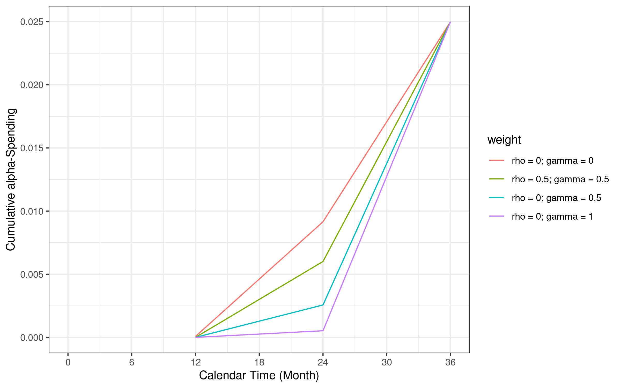
The table below provide the cumulative alpha and beta at different analysis time for each WLR test.

we draw the Alpha spending (\(\alpha=0.025\)) function based on information fraction at 12, 24 and 36 months

Similarly, we draw the Beta spending (\(\beta=0.2\)) function based on information fraction at 12, 24 and 36 months

analysisTimes <- c(12, 24, 36)
gs_spend <- lapply(weight_fun, function(weight) {
  tmp <- gsdmvn::gs_info_wlr(
    enrollRates, failRates,
    analysisTimes = analysisTimes,
    weight = weight
  )

  tmp %>% mutate(
    theta = abs(delta) / sqrt(sigma2),
    info = info / max(info),
    info0 = info0 / max(info0),
    alpha = gsDesign::sfLDOF(alpha = 0.025, t = info0)$spend,
    beta = gsDesign::sfLDOF(alpha = 0.20, t = info)$spend
  )
})

names(gs_spend) <- weight_name
bind_rows(gs_spend, .id = "weight") %>%
  select(weight, Time, alpha, beta) %>%
  mutate_if(is.numeric, round, digits = 3)

#>                    weight Time alpha  beta
#> 1      rho = 0; gamma = 0   12 0.000 0.025
#> 2      rho = 0; gamma = 0   24 0.009 0.139
#> 3      rho = 0; gamma = 0   36 0.025 0.200
#> 4  rho = 0.5; gamma = 0.5   12 0.000 0.003
#> 5  rho = 0.5; gamma = 0.5   24 0.006 0.118
#> 6  rho = 0.5; gamma = 0.5   36 0.025 0.200
#> 7    rho = 0; gamma = 0.5   12 0.000 0.000
#> 8    rho = 0; gamma = 0.5   24 0.003 0.088
#> 9    rho = 0; gamma = 0.5   36 0.025 0.200
#> 10     rho = 0; gamma = 1   12 0.000 0.000
#> 11     rho = 0; gamma = 1   24 0.001 0.051
#> 12     rho = 0; gamma = 1   36 0.025 0.200

8.5 Lower and upper bound

Let’s calculate the lower and upper bound of the first interim analysis.

First interim analysis upper bound: \(\text{Pr}(Z_1 > b_1 \mid H_0)\)

-qnorm(gs_spend[[1]]$alpha[1])

#> [1] 3.790778

First interim analysis lower bound \(\text{Pr}(Z_1 < b_1 \mid H_1)\)

The lower bound is calculated under alternative hypothesis and depends on sample size.

n <- 400
mean <- gs_spend[[1]]$theta[1] * sqrt(n)
qnorm(gs_spend[[1]]$beta[1], mean = mean, sd = 1)

#> [1] -1.159606

n <- 500
mean <- gs_spend[[1]]$theta[1] * sqrt(n)
qnorm(gs_spend[[1]]$beta[1], mean = mean, sd = 1)

#> [1] -1.065469

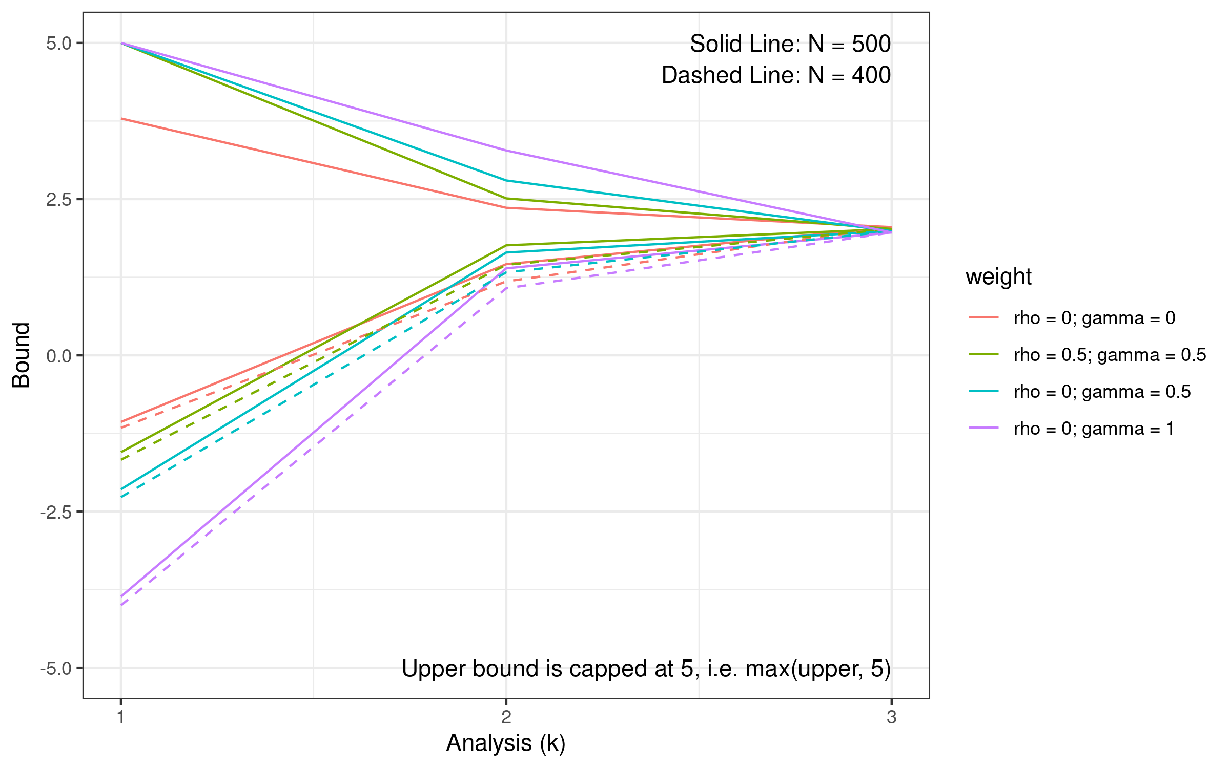
The figure below illustrates the lower and upper bound in different sample size

A larger sample size has a larger lower bound (solid line compared with dashed line)
Iteration is required to find proper sample size and boundary.

8.6 Sample size calculation logrank test based on AHR

Sample size

x <- gsdmvn::gs_design_ahr(
  enrollRates = enrollRates, failRates = failRates,
  ratio = ratio, alpha = alpha, beta = beta,
  upper = gs_spending_bound,
  lower = gs_spending_bound,
  upar = list(sf = gsDesign::sfLDOF, total_spend = alpha),
  lpar = list(sf = gsDesign::sfLDOF, total_spend = beta),
  analysisTimes = analysisTimes
)$bounds %>%
  mutate_if(is.numeric, round, digits = 2)
x

#> # A tibble: 6 × 11
#>   Analysis Bound  Time     N Events     Z Probability   AHR theta  info info0
#>      <dbl> <chr> <dbl> <dbl>  <dbl> <dbl>       <dbl> <dbl> <dbl> <dbl> <dbl>
#> 1        1 Upper    12  379.   81.4  3.77        0     0.84  0.17  20.0  20.3
#> 2        2 Upper    24  379.  187.   2.35        0.47  0.71  0.34  45.5  46.6
#> 3        3 Upper    36  379.  251.   2.01        0.8   0.68  0.38  61.6  62.7
#> 4        1 Lower    12  379.   81.4 -1.19        0.02  0.84  0.17  20.0  20.3
#> 5        2 Lower    24  379.  187.   1.13        0.14  0.71  0.34  45.5  46.6
#> 6        3 Lower    36  379.  251.   2.01        0.2   0.68  0.38  61.6  62.7

Simulation results based on 10,000 replications.

#>     n  t events  ahr lower upper
#> 1 379 12  81.23 0.86  0.02  0.00
#> 2 379 24 186.50 0.72  0.13  0.48
#> 3 379 36 251.05 0.69  0.19  0.81

Type I error

gsdmvn::gs_power_npe(
  theta = rep(0, length(analysisTimes)),
  info = x$info0[x$Bound == "Upper"],
  upar = x$Z[x$Bound == "Upper"],
  lpar = rep(-Inf, 3)
)$Probability[1:length(analysisTimes)]

#> [1] 8.162377e-05 9.415389e-03 2.505418e-02

Compared with fixed design

gsdmvn::gs_design_ahr(
  enrollRates = enrollRates, failRates = failRates,
  ratio = 1, alpha = 0.025, beta = 0.2,
  upar = -qnorm(0.025),
  lpar = -qnorm(0.025),
  analysisTimes = 36
)$bounds

#> # A tibble: 1 × 11
#>   Analysis Bound  Time     N Events     Z Probability   AHR theta  info info0
#>      <dbl> <chr> <dbl> <dbl>  <dbl> <dbl>       <dbl> <dbl> <dbl> <dbl> <dbl>
#> 1        1 Upper    36  328.   217.  1.96         0.8 0.683 0.381  53.4  54.4

8.7 Sample size calculation logrank test based on WLR \(FH(0, 0)\)

Sample size

x <- gsdmvn::gs_design_wlr(
  enrollRates = enrollRates, failRates = failRates,
  ratio = ratio, alpha = alpha, beta = beta,
  weight = function(x, arm0, arm1) {
    gsdmvn::wlr_weight_fh(x, arm0, arm1, rho = 0, gamma = 0)
  },
  upper = gs_spending_bound,
  lower = gs_spending_bound,
  upar = list(sf = gsDesign::sfLDOF, total_spend = alpha),
  lpar = list(sf = gsDesign::sfLDOF, total_spend = beta),
  analysisTimes = analysisTimes
)$bounds %>%
  mutate_if(is.numeric, round, digits = 2)
x

#> # A tibble: 6 × 11
#>   Analysis Bound  Time     N Events     Z Probability   AHR theta  info info0
#>      <dbl> <chr> <dbl> <dbl>  <dbl> <dbl>       <dbl> <dbl> <dbl> <dbl> <dbl>
#> 1        1 Upper    12  377.    81   3.79        0     0.84  0.17  20.2  20.3
#> 2        2 Upper    24  377.   186.  2.36        0.46  0.72  0.33  46.3  46.8
#> 3        3 Upper    36  377.   250.  2.01        0.8   0.68  0.38  61.8  63.3
#> 4        1 Lower    12  377.    81  -1.18        0.03  0.84  0.17  20.2  20.3
#> 5        2 Lower    24  377.   186.  1.15        0.14  0.72  0.33  46.3  46.8
#> 6        3 Lower    36  377.   250.  2.01        0.2   0.68  0.38  61.8  63.3

Simulation results based on 10,000 replications.

#>     n  t events  ahr lower upper
#> 1 378 12  80.98 0.86  0.03  0.00
#> 2 378 24 186.10 0.72  0.14  0.47
#> 3 378 36 250.33 0.69  0.20  0.80

Type I error

gsdmvn::gs_power_npe(
  theta = rep(0, length(analysisTimes)),
  info = x$info0[x$Bound == "Upper"],
  upar = x$Z[x$Bound == "Upper"],
  lpar = rep(-Inf, 3)
)$Probability[1:length(analysisTimes)]

#> [1] 7.532364e-05 9.164191e-03 2.497474e-02

Compared with fixed design

gsdmvn::gs_design_wlr(
  enrollRates = enrollRates, failRates = failRates,
  weight = function(x, arm0, arm1) {
    gsdmvn::wlr_weight_fh(x, arm0, arm1, rho = 0, gamma = 0)
  },
  ratio = 1, alpha = 0.025, beta = 0.2,
  upar = -qnorm(0.025),
  lpar = -qnorm(0.025),
  analysisTimes = 36
)$bounds

#> # A tibble: 1 × 11
#>   Analysis Bound  Time     N Events     Z Probability   AHR theta  info info0
#>      <dbl> <chr> <dbl> <dbl>  <dbl> <dbl>       <dbl> <dbl> <dbl> <dbl> <dbl>
#> 1        1 Upper    36  324.   215.  1.96         0.8 0.683 0.381  53.2  54.5

8.8 Sample size calculation \(FH(0, 1)\)

Sample size

x <- gsdmvn::gs_design_wlr(
  enrollRates = enrollRates, failRates = failRates,
  ratio = ratio, alpha = alpha, beta = beta,
  weight = function(x, arm0, arm1) {
    gsdmvn::wlr_weight_fh(x, arm0, arm1, rho = 0, gamma = 1)
  },
  upper = gs_spending_bound,
  lower = gs_spending_bound,
  upar = list(sf = gsDesign::sfLDOF, total_spend = alpha),
  lpar = list(sf = gsDesign::sfLDOF, total_spend = beta),
  analysisTimes = analysisTimes
)$bounds %>%
  mutate_if(is.numeric, round, digits = 2)
x

#> # A tibble: 6 × 11
#>   Analysis Bound  Time     N Events      Z Probability   AHR theta  info info0
#>      <dbl> <chr> <dbl> <dbl>  <dbl>  <dbl>       <dbl> <dbl> <dbl> <dbl> <dbl>
#> 1        1 Upper    12  287.   61.6 Inf           0     0.73  1.58  0.4   0.41
#> 2        2 Upper    24  287.  141.    3.28        0.16  0.64  1.33  2.99  3.1 
#> 3        3 Upper    36  287.  190.    1.96        0.8   0.62  1.08  6.95  7.43
#> 4        1 Lower    12  287.   61.6  -4.18        0     0.73  1.58  0.4   0.41
#> 5        2 Lower    24  287.  141.    0.66        0.05  0.64  1.33  2.99  3.1 
#> 6        3 Lower    36  287.  190.    1.96        0.2   0.62  1.08  6.95  7.43

Simulation results based on 10,000 replications.

#>      n  t events  ahr lower upper
#> 10 287 12  61.64 0.77  0.00  0.00
#> 11 287 24 141.41 0.65  0.05  0.17
#> 12 287 36 190.20 0.63  0.20  0.80

Type I error

gsdmvn::gs_power_npe(
  theta = rep(0, length(analysisTimes)),
  info = x$info0[x$Bound == "Upper"],
  upar = x$Z[x$Bound == "Upper"],
  lpar = rep(-Inf, 3)
)$Probability[1:length(analysisTimes)]

#> [1] 0.0000000000 0.0005191052 0.0251730067

Compared with fixed design

gsdmvn::gs_design_wlr(
  enrollRates = enrollRates, failRates = failRates,
  weight = function(x, arm0, arm1) {
    gsdmvn::wlr_weight_fh(x, arm0, arm1, rho = 0, gamma = 1)
  },
  ratio = 1, alpha = 0.025, beta = 0.2,
  upar = -qnorm(0.025),
  lpar = -qnorm(0.025),
  analysisTimes = 36
)$bounds

#> # A tibble: 1 × 11
#>   Analysis Bound  Time     N Events     Z Probability   AHR theta  info info0
#>      <dbl> <chr> <dbl> <dbl>  <dbl> <dbl>       <dbl> <dbl> <dbl> <dbl> <dbl>
#> 1        1 Upper    36  264.   175.  1.96         0.8 0.617  1.08  6.41  6.85

8.9 Sample size calculation \(FH(0, 0.5)\)

Sample size

x <- gsdmvn::gs_design_wlr(
  enrollRates = enrollRates, failRates = failRates,
  ratio = ratio, alpha = alpha, beta = beta,
  weight = function(x, arm0, arm1) {
    gsdmvn::wlr_weight_fh(x, arm0, arm1, rho = 0, gamma = 0.5)
  },
  upper = gs_spending_bound,
  lower = gs_spending_bound,
  upar = list(sf = gsDesign::sfLDOF, total_spend = alpha),
  lpar = list(sf = gsDesign::sfLDOF, total_spend = beta),
  analysisTimes = analysisTimes
)$bounds %>%
  mutate_if(is.numeric, round, digits = 2)
x

#> # A tibble: 6 × 11
#>   Analysis Bound  Time     N Events     Z Probability   AHR theta  info info0
#>      <dbl> <chr> <dbl> <dbl>  <dbl> <dbl>       <dbl> <dbl> <dbl> <dbl> <dbl>
#> 1        1 Upper    12  288.   61.9  6.18        0     0.78  0.63  2.08  2.09
#> 2        2 Upper    24  288.  142    2.8         0.3   0.67  0.77  8.86  9.07
#> 3        3 Upper    36  288.  191.   1.97        0.8   0.64  0.73 15.7  16.4 
#> 4        1 Lower    12  288.   61.9 -2.43        0     0.78  0.63  2.08  2.09
#> 5        2 Lower    24  288.  142    0.93        0.09  0.67  0.77  8.86  9.07
#> 6        3 Lower    36  288.  191.   1.97        0.2   0.64  0.73 15.7  16.4

Simulation results based on 10,000 replications.

#>     n  t events  ahr lower upper
#> 7 289 12  62.11 0.81  0.00   0.0
#> 8 289 24 142.28 0.68  0.09   0.3
#> 9 289 36 191.44 0.65  0.20   0.8

Type I error

gsdmvn::gs_power_npe(
  theta = rep(0, length(analysisTimes)),
  info = x$info0[x$Bound == "Upper"],
  upar = x$Z[x$Bound == "Upper"],
  lpar = rep(-Inf, 3)
)$Probability[1:length(analysisTimes)]

#> [1] 3.205080e-10 2.555246e-03 2.523428e-02

Compared with fixed design

gsdmvn::gs_design_wlr(
  enrollRates = enrollRates, failRates = failRates,
  weight = function(x, arm0, arm1) {
    gsdmvn::wlr_weight_fh(x, arm0, arm1, rho = 0, gamma = 0.5)
  },
  ratio = 1, alpha = 0.025, beta = 0.2,
  upar = -qnorm(0.025),
  lpar = -qnorm(0.025),
  analysisTimes = 36
)$bounds

#> # A tibble: 1 × 11
#>   Analysis Bound  Time     N Events     Z Probability   AHR theta  info info0
#>      <dbl> <chr> <dbl> <dbl>  <dbl> <dbl>       <dbl> <dbl> <dbl> <dbl> <dbl>
#> 1        1 Upper    36  261.   173.  1.96         0.8 0.639 0.732  14.2  14.9

8.10 Sample size calculation \(FH(0.5, 0.5)\)

Sample size

x <- gsdmvn::gs_design_wlr(
  enrollRates = enrollRates, failRates = failRates,
  ratio = ratio, alpha = alpha, beta = beta,
  weight = function(x, arm0, arm1) {
    gsdmvn::wlr_weight_fh(x, arm0, arm1, rho = 0.5, gamma = 0.5)
  },
  upper = gs_spending_bound,
  lower = gs_spending_bound,
  upar = list(sf = gsDesign::sfLDOF, total_spend = alpha),
  lpar = list(sf = gsDesign::sfLDOF, total_spend = beta),
  analysisTimes = analysisTimes
)$bounds %>%
  mutate_if(is.numeric, round, digits = 2)
x

#> # A tibble: 6 × 11
#>   Analysis Bound  Time     N Events     Z Probability   AHR theta  info info0
#>      <dbl> <chr> <dbl> <dbl>  <dbl> <dbl>       <dbl> <dbl> <dbl> <dbl> <dbl>
#> 1        1 Upper    12  304.   65.3  5.05        0     0.79  0.68  1.76  1.77
#> 2        2 Upper    24  304.  150.   2.51        0.42  0.68  0.93  6.17  6.28
#> 3        3 Upper    36  304.  201.   1.99        0.8   0.65  0.97  9.16  9.44
#> 4        1 Lower    12  304.   65.3 -1.8         0     0.79  0.68  1.76  1.77
#> 5        2 Lower    24  304.  150.   1.12        0.12  0.68  0.93  6.17  6.28
#> 6        3 Lower    36  304.  201.   1.99        0.2   0.65  0.97  9.16  9.44

Simulation results based on 10,000 replications.

load("simulation/simu_gsd_wlr_boundary.Rdata")
simu_res %>%
  subset(rho == 0.5 & gamma == 0.5) %>%
  select(-scenario, -rho, -gamma) %>%
  mutate_if(is.numeric, round, digits = 2)

#>     n  t events  ahr lower upper
#> 4 304 12  65.10 0.81  0.00  0.00
#> 5 304 24 149.51 0.68  0.12  0.42
#> 6 304 36 201.23 0.66  0.20  0.80

Type I error

gsdmvn::gs_power_npe(
  theta = rep(0, length(analysisTimes)),
  info = x$info0[x$Bound == "Upper"],
  upar = x$Z[x$Bound == "Upper"],
  lpar = rep(-Inf, 3)
)$Probability[1:length(analysisTimes)]

#> [1] 2.209050e-07 6.036759e-03 2.515345e-02

Compared with fixed design

gsdmvn::gs_design_wlr(
  enrollRates = enrollRates, failRates = failRates,
  weight = function(x, arm0, arm1) {
    gsdmvn::wlr_weight_fh(x, arm0, arm1, rho = 0.5, gamma = 0.5)
  },
  ratio = 1, alpha = 0.025, beta = 0.2,
  upar = -qnorm(0.025),
  lpar = -qnorm(0.025),
  analysisTimes = 36
)$bounds

#> # A tibble: 1 × 11
#>   Analysis Bound  Time     N Events     Z Probability   AHR theta  info info0
#>      <dbl> <chr> <dbl> <dbl>  <dbl> <dbl>       <dbl> <dbl> <dbl> <dbl> <dbl>
#> 1        1 Upper    36  269.   178.  1.96         0.8 0.650 0.973  8.11  8.36

7 Weighted logrank test

9 MaxCombo test