4 Introduction to gsdmvn, gsDesign2, and simtrial

simtrial, gsDesign2 and gsdmvn are under development and hosted on GitHub/Merck. Below is the Github repo link to the source code

• simtrial: https://github.com/Merck/simtrial
• gsDesign2: https://github.com/Merck/gsDesign2
• gsdmvn: https://github.com/Merck/gsdmvn

Note: As of June 14, 2023, the gsdmvn package has been integrated into the gsDesign2 package and archived on GitHub. For future projects, we recommend using gsDesign2 (now available from CRAN) directly. Despite the fact that the code within this material has not been updated, it remains functional provided you install the specific development versions detailed in the preface.

4.1 simtrial

The R package simtrial targets on time-to-event trial simulation under the piecewise model. It uses logrank and weighted logrank for analysis. It can simulate both fixed and group sequential design, also potential to simulate adaptive design. Its validation is near completion (thanks to AP colleagues and Amin Shirazi).

In simtrial, there are several functions to generate simulated datasets:

• simfix(): Simulation of fixed sample size design for time-to-event endpoint
• simfix2simPWSurv(): Conversion of enrollment and failure rates from simfix() to simPWSurv() format
• simPWSurv(): Simulate a stratified time-to-event outcome randomized trial

There are also functions to cut data for analysis:

• cutData(): Cut a dataset for analysis at a specified date
• cutDataAtCount(): Cut a dataset for analysis at a specified event count
• getCutDateForCount(): Get date at which an event count is reached

Most importantly, there are functions for analysis:

• tenFH(): Fleming-Harrington weighted logrank tests
• tenFHcorr(): Fleming-Harrington weighted logrank tests plus correlations
• tensurv(): Process survival data into counting process format
• pMaxCombo(): MaxCombo p-value
• pwexpfit(): Piecewise exponential survival estimation
• wMB(): Magirr and Burman modestly weighted logrank tests

In simtrial, there are reverse engineered datasets:

• Ex1delayedEffect: Time-to-event data example 1 for non-proportional hazards working group
• Ex2delayedEffect: Time-to-event data example 2 for non-proportional hazards working group
• Ex3curewithph: Time-to-event data example 3 for non-proportional hazards working group
• Ex4belly: Time-to-event data example 4 for non-proportional hazards working group
• Ex5widening: Time-to-event data example 5 for non-proportional hazards working group
• Ex6crossing: Time-to-event data example 6 for non-proportional hazards working group
• MBdelayed: Simulated survival dataset with delayed treatment effect

4.2 gsDesign2

The R package gsDesign2 has the main functions listed as follows.

• AHR(): Average hazard ratio under non-proportional hazards
• eAccrual(): Piecewise constant expected accrual
• eEvents_df(): Expected events observed under piecewise exponential model
• ppwe(): Estimate piecewise exponential cumulative distribution function
• s2pwe(): Approximate survival distribution with piecewise exponential distribution
• tEvents(): Predict time at which a targeted event count is achieved

4.3 gsdmvn

The R package gsdmvn extends the Jennison and Turnbull (2000) computational model to non-constant treatment effects. The bound supports functions include

• gs_b(): direct input of bounds;
• gs_spending_bound(): spending function bounds.

Besides, it covers three models for analysis.

• Average hazard ratio model (see detailed description in Section 3.2)
  • gs_power_ahr(): Power computation
  • gs_design_ahr(): Design computations
• Weighted logrank model (see detailed description in Section 7)
  • gs_power_wlr(): Power computation
  • gs_design_wlr(): Design computations
• MaxCombo model (see detailed description in Section 9)
  • gs_power_combo(): Power computation
  • gs_design_combo(): Design computations

4.4 Simulation

In this section, we conduct three simulations.

The first simulation is to compare the simulated power and asymptotic power. Specifically speaking, we compare the results from gsdmvn::gs_power_ahr() with that from simtrial::simfix(). The details of this simulation can be found in Section 4.4.1.

The second simulation is to compare the simulated power and asymptotic power. Specifically speaking, we compare the results from gsDesign2::AHR() with that from simtrial::simPWSurv(). The details of this simulation can be found in Section 4.4.2.

The third simulation is to compare the estimation of \(\beta\) by MLE and weighted summation as in Section 3.2. The details of this simulation can be found in Section 4.4.3.

4.4.1 Simulation 1: Compare the IA power by gs_power_ahr() and simulation sim_fix()

This section compares the simulated power and asymptotic power. The simulated power is calculated by simtrial::simfix(), and the asymptotic power is calculated by gsdmvn::gs_power_ahr(). To conduct the comparison, we first save the output of simtrial::simfix() by running the following code chunk. After that, we simply load the simulation results and compare it with the asymptotic power.

library(gsDesign)
library(simtrial)
library(dplyr)
library(gsdmvn)

## Set the enrollment rates
my_enrollRates <- tibble::tibble(
  Stratum = "All",
  duration = c(2, 2, 2, 6),
  rate = c(6, 12, 18, 24)
)
## Set the failure rates
my_failRates <- tibble::tibble(
  Stratum = "All",
  duration = 1,
  failRate = log(2) / 9,
  hr = 0.65,
  dropoutRate = 0.001
)
## Set the number of simulations
my_nsim <- 1e+5

## Create a group sequential design for survival outcome
my_gsSurv <- gsSurv(
  k = 2,
  test.type = 1,
  alpha = 0.025,
  beta = 0.2,
  astar = 0,
  timing = 0.7,
  sfu = sfLDOF,
  sfupar = c(0),
  sfl = sfLDOF,
  sflpar = c(0),
  lambdaC = log(2) / 9,
  hr = 0.65,
  hr0 = 1,
  eta = 0.001,
  gamma = c(6, 12, 18, 24),
  R = c(2, 2, 2, 6),
  S = NULL,
  T = NULL,
  minfup = NULL,
  ratio = 1
)

# Update my_gsSurv with gsDesign() to get integer event counts
my_gsDesign <- gsDesign(
  k = my_gsSurv$k,
  test.type = 1,
  alpha = my_gsSurv$alpha,
  beta = my_gsSurv$beta,
  sfu = my_gsSurv$upper$sf,
  sfupar = my_gsSurv$upper$param,
  n.I = ceiling(my_gsSurv$n.I),
  maxn.IPlan = ceiling(my_gsSurv$n.I[my_gsSurv$k]),
  delta = my_gsSurv$delta,
  delta1 = my_gsSurv$delta1,
  delta0 = my_gsSurv$delta0
)

set.seed(123)
my_simfix <- simfix( # Number of simulations to perform.
  nsim = my_nsim,
  # Total sample size per simulation.
  sampleSize = ceiling(max(my_gsSurv$eNC) + max(my_gsSurv$eNE)),
  # A tibble with
  # (1) strata specified in `Stratum`
  # (2) probability (incidence) of each stratum in `p`.
  strata = tibble::tibble(Stratum = "All", p = 1),
  # Targeted event count for analysis.
  # Here we only target on the 1st IA only.
  targetEvents = my_gsDesign$n.I[1],
  # Vector of treatments to be included in each block
  block = c(rep("Control", 2), rep("Experimental", 2)),
  # Piecewise constant enrollment rates by time period.
  enrollRates = my_enrollRates,
  # Piecewise constant control group failure rates,
  # hazard ratio for experimental vs control,
  # and dropout rates by stratum and time period.
  failRates = my_failRates,
  # `timingType` has up to 5 elements indicating different options for data cutoff.
  # `timingType = 1`: uses the planned study duration
  # `timingType = 2`: the time the targeted event count is achieved
  # `timingType = 3`: the planned minimum follow-up after enrollment is complete
  # `timingType = 4`: the maximum of planned study duration and targeted event count cuts (1 and 2)
  # `timingType = 5`: the maximum of targeted event count and minimum follow-up cuts (2 and 3)
  timingType = 2
)
# Save the simulation data
save(my_gsDesign, file = "./data/simulation_gs_power_ahr_my_gsDesign.Rdata")
save(my_simfix, file = "./data/simulation_gs_power_ahr_my_simfix.Rdata")

library(gsDesign)
library(simtrial)
library(dplyr)
library(gsdmvn)

load("./data/simulation_gs_power_ahr_my_simfix.Rdata")
load("./data/simulation_gs_power_ahr_my_gsDesign.Rdata")

## Set the enrollment rates
my_enrollRates <- tibble::tibble(
  Stratum = "All",
  duration = c(2, 2, 2, 6),
  rate = c(6, 12, 18, 24)
)
## Set the failure rates
my_failRates <- tibble::tibble(
  Stratum = "All",
  duration = 1,
  failRate = log(2) / 9,
  hr = 0.65,
  dropoutRate = 0.001
)
my_nsim <- 1e+5

# Calculate the simulated power at the 1st IA
my_sim_IA_power <- as.numeric(my_simfix %>% summarize(mean(Z <= -my_gsDesign$upper$bound[1])))

# Calculate the power by gs_ahr_power() at the 1st IA
out <- gs_power_ahr(
  enrollRates = my_enrollRates,
  failRates = my_failRates,
  ratio = 1,
  events = my_gsDesign$n.I, # set number of events the same as my_gsDesign above from gsDesign()
  analysisTimes = NULL,
  binding = FALSE,
  upper = gs_spending_bound,
  upar = list(sf = gsDesign::sfLDOF, total_spend = 0.025, param = NULL, timing = NULL, theta = 0),
  lower = gs_spending_bound,
  lpar = list(sf = gsDesign::sfLDOF, total_spend = 0.2, param = NULL, timing = NULL, theta = 0),
  test_upper = TRUE,
  test_lower = FALSE
)
my_ahr_IA_power <- out$Probability[1]

cat("The power at the 1st IA by gs_power_ahr() is:", my_ahr_IA_power, "\n")

#> The power at the 1st IA by gs_power_ahr() is: 0.4605649

cat("The power at the 1st IA by", my_nsim, "simulation is:", my_sim_IA_power, "\n")

#> The power at the 1st IA by 1e+05 simulation is: 0.46655

4.4.2 Simulation 2: Compare AHR by gsDesign2::AHR() and simtrial::simPWSurv()

This section compares the simulated AHR and asymptotic AHR The simulated power is calculated by simtrial::simPWSurv(), and the asymptotic power is calculated by gsDesign2::AHR(). To conduct the comparison, we first save the output of simtrial::simPWSurv() by running the following code chunk. After that, we simply load the simulation results and compare it with the asymptotic AHR

library(survival)
library(dplyr)
library(simtrial)

# Set the sample size
my_N <- 500
# Set the analysis time, i.e., there are 4 looks
my_analysisTimes <- c(12, 20, 28, 36)
# Set the enrollment rates
# This format of enrollment rates is design for simtrial::simfix()
# If it is later used to simtrial::simPWSurv(),
# function simtrial::simfix2simPWSurv() can used for transformation
my_enrollRates <- tibble(
  Stratum = "All",
  duration = 12,
  rate = my_N / 12
)
# Set the failure rates
# This format of failure rates is design for simtrial::simfix()
# If it is later used to simtrial::simPWSurv(),
# function simtrial::simfix2simPWSurv() can used for transformation
my_failRates <- tibble(
  Stratum = "All",
  duration = c(4, 100),
  failRate = log(2) / 15,
  hr = c(1, 0.6),
  dropoutRate = 0.001
)

# Set number of simulations
my_nsim <- 10
# Set up matrix for simulation results
results <- matrix(0, nrow = my_nsim * 4, ncol = 6)
colnames(results) <- c("Sim", "Analysis", "Events", "beta", "var", "logrank")

# Set the index for results row
ii <- 1
set.seed(123)
for (sim in 1:my_nsim) {
  # Simulate a trial
  ds <- simPWSurv( # Generate my_N observations
    n = my_N,
    # Use the same enrollRates as that in AHR
    enrollRates = my_enrollRates,
    # Conversion of failRates from simfix() to simPWSurv() format
    failRates = simfix2simPWSurv(my_failRates)$failRates,
    # Conversion of dropoutRates from simfix() to simPWSurv() format
    dropoutRates = simfix2simPWSurv(my_failRates)$dropoutRates
  )
  # For each generated my_N observations
  # Go through pre-defined 4 looks
  for (j in seq_along(my_analysisTimes)) {
    # Cut data at specified analysis times
    # Use cutDataAtCount to cut at event count
    # des is a dataset ready for survival analysis
    dsc <- ds %>% cutData(my_analysisTimes[j])

    # 1st column of results records the index of the simulation
    results[ii, 1] <- sim
    # 2nd column of results records the index of the look
    results[ii, 2] <- j
    # 3rd column of results records the number of events
    results[ii, 3] <- sum(dsc$event)

    # Apply Cox model
    cox <- coxph(Surv(tte, event) ~ Treatment, data = dsc)
    # 4th column of results records the number log HR
    results[ii, 4] <- as.numeric(cox$coefficients)
    # 5th column of results records the variance
    results[ii, 5] <- as.numeric(cox$var)

    # Logrank test
    Z <- dsc %>%
      tensurv(txval = "Experimental") %>%
      tenFH(rg = tibble::tibble(rho = 0, gamma = 0))
    # 5th column of results records the logrank
    results[ii, 6] <- as.numeric(Z$Z)

    # Increate the row index
    ii <- ii + 1
  }
}
save(results, file = "./data/simulation_AHR_simPRSurv.Rdata")

# Calculate the simulated AHR
load("./data/simulation_AHR_simPRSurv.Rdata")

# Distribution of Cox coefficient
ggplot(tibble::as_tibble(results), 
       aes(x = factor(Analysis), y = beta)) +
  geom_violin() +
  ggtitle("Distribution of Cox Coefficient by Analysis") +
  xlab("Analysis") +
  ylab("Cox coefficient")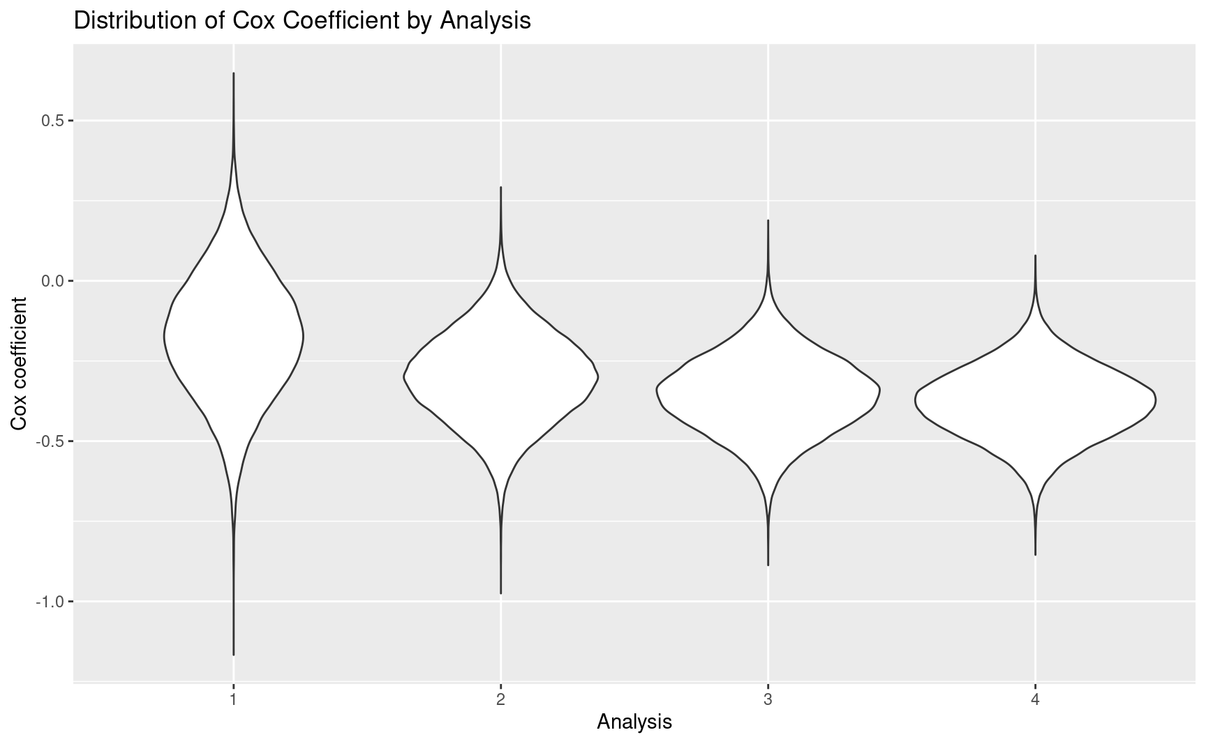

# Variability of results
library(dplyr)
ggplot(filter(tibble::as_tibble(results), Sim < 10) %>% 
         mutate(Sim = factor(Sim), Analysis = factor(Analysis)), 
       aes(x = Analysis, y = exp(beta), group = Sim, col = Sim)) +
  geom_line(show.legend = FALSE) +
  geom_point(aes(shape = Analysis), show.legend = FALSE) +
  scale_y_log10(breaks = seq(.6, 1.1, .1)) +
  ylab("HR")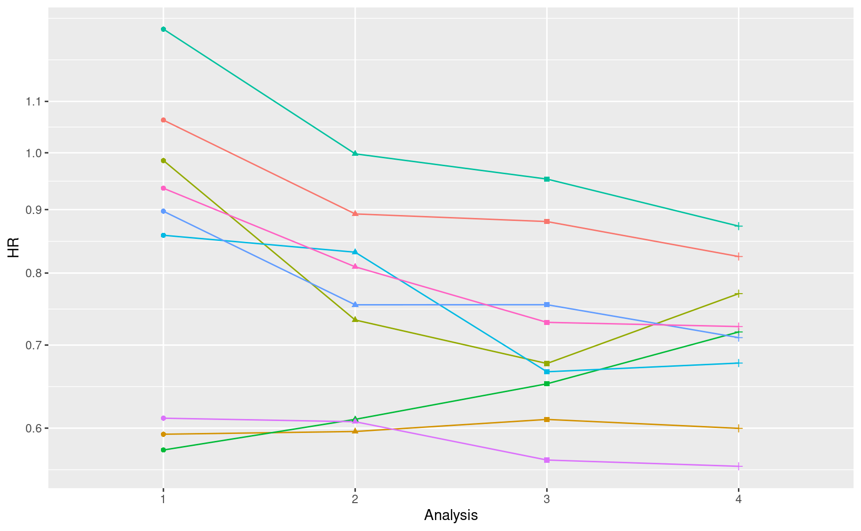

# Comparison of asymptotic vs simulation
AHR_simulated <- tibble::as_tibble(results) %>%
  group_by(Analysis) %>%
  summarize(
    AHR = exp(mean(beta)),
    Events = mean(Events),
    info = 1 / mean(var(beta)),
    info0 = Events / 4
  ) %>%
  select(AHR, Events, info, info0)
colnames(AHR_simulated) <- c("AHR_sim", "Events_sim", "info_sim", "info0_sim")

# Calculate the AHR asymptotically
# gsDesign2::AHR() uses asymptotic distribution
# We will compare its outputs with the simulated outputs
# The simulated outputs is calculated by simtrial::simPWSurv()

# Set the sample size the same as simPWSurv()
my_N <- 500
# Set the analysis time the same as simPWSurv()
my_analysisTimes <- c(12, 20, 28, 36)
# Set the enrollment rates the same as simPWSurv()
my_enrollRates <- tibble(
  Stratum = "All",
  duration = 12,
  rate = my_N / 12
)
# Set the failure rates the same as simPWSurv()
my_failRates <- tibble(
  Stratum = "All",
  duration = c(4, 100),
  failRate = log(2) / 15,
  hr = c(1, 0.6),
  dropoutRate = 0.001
)

AHR_asymptotics <- gsDesign2::AHR(
  enrollRates = my_enrollRates,
  failRates = my_failRates,
  totalDuration = my_analysisTimes,
  ratio = 1
)
colnames(AHR_asymptotics) <- c("Time", "AHR_asy", "Events_asy", "info_asy", "info0_asy")

# Compare the results
cbind(AHR_asymptotics, AHR_simulated) %>%
  gt::gt() %>%
  gt::fmt_number(columns = c(2, 4, 5, 6, 8, 9), decimals = 4) %>%
  gt::fmt_number(columns = c(3, 7), decimals = 2)

Time	AHR_asy	Events_asy	info_asy	info0_asy	AHR_sim	Events_sim	info_sim	info0_sim
12	0.8395	107.39	26.3710	26.8486	0.8415	107.25	26.2593	26.8130
20	0.7379	207.90	50.6695	51.9741	0.7397	207.71	50.8936	51.9281
28	0.7000	279.10	68.2263	69.7759	0.7012	278.93	67.9878	69.7321
36	0.6832	331.29	81.3779	82.8227	0.6839	331.19	80.6198	82.7969

4.4.3 Simulation 3: Compare \(\beta\) by MLE and weighted summation

This section compares the AHR estimated by MLE (see theoretical details in Section ??) and weighted summation (see theoretical details in Section ??).

library(dplyr)
library(gt)
my_nsim <- 10
my_nNewtonRaphson <- 10
compare_results <- matrix(0, nrow = my_nsim, ncol = 2)
set.seed(123)

for (sim in 1:my_nsim) {
  # Generate the number of change points, i.e., total number of timeline piece - 1
  sim_M <- sample(3:10, size = 1)
  sim_d0_start <- sample(4:8, size = 1)
  sim_d1_start <- sim_d0_start - 3
  sim_T0_start <- sample(10:20, size = 1)
  sim_T1_start <- sim_T0_start + 1
  # Generate simulated data
  obs_data <- data.frame( # m = 1:5,
    m = sim_M,
    # d0 = 4:8,
    d0 = seq(from = sim_d0_start, length.out = sim_M),
    # d1 = 1:5,
    d1 = seq(from = sim_d1_start, length.out = sim_M),
    # T0 = 10:14,
    T0 = seq(from = sim_T0_start, length.out = sim_M),
    # T1 = 11:15
    T1 = seq(from = sim_T1_start, length.out = sim_M)
  ) %>%
    mutate(
      lambda0 = d0 / T0,
      lambda1 = d1 / T1,
      HR = lambda1 / lambda0,
      # beta_m
      gamma = log(HR),
      # Var(beta_m)
      vargamma = 1 / d0 + 1 / d1
    )

  # Estimate beta by weighted summation
  # beta = variable `logAHR`
  estimate_beta_WS <- obs_data %>%
    summarise(
      wsum = sum(1 / vargamma),
      # estimation of beta_WS
      beta_WS = sum(gamma / vargamma) / wsum,
      # variance of the estimation of beta_WS
      var = sum(vargamma^(-1))^(-1),
      # standard derivation of the estimation of beta_WS
      se = sqrt(var),
      # AHR: average of lambda_{1,m}/lambda_{0,m}
      AHR = exp(beta_WS)
    )
  compare_results[sim, 1] <- estimate_beta_WS$beta_WS

  # Estimate beta by MLE
  beta_MLE <- estimate_beta_WS$beta_WS
  # beta_MLE_seq <- beta_MLE    # ensure convergence

  for (i in 1:my_nNewtonRaphson) {
    ## Calculate the first order derivative at the value of beta_k
    temp_beta_d1 <- obs_data %>%
      summarise(beta_d1 = -sum((d0 + d1) * T1 * exp(beta_MLE) / (T0 + T1 * exp(beta_MLE)))
      +
        sum(d1))
    beta_d1_curr <- temp_beta_d1$beta_d1

    ## Calculate the second order derivative at the value of beta_k
    temp_beta_d2 <- obs_data %>%
      summarise(beta_d2 = sum((T1 * exp(beta_MLE))^2 * (d0 + d1) / (T0 + T1 * exp(beta_MLE))^2)
      -
        sum(((d0 + d1) * T1 * exp(beta_MLE)) / (T0 + T1 * exp(beta_MLE))))
    beta_d2_curr <- temp_beta_d2$beta_d2

    ## Update beta by Newton-Raphson method, i.e.,
    ## beta_k+1 = beta_k - l'(beta_k)/l''(beta_k)
    beta_MLE <- beta_MLE - beta_d1_curr / beta_d2_curr
    # beta_MLE_seq <- c(beta_MLE_seq, beta_MLE)
  }

  compare_results[sim, 2] <- beta_MLE
}

colnames(compare_results) <- c("Weighted Summation", "MLE")
save(compare_results, file = "./data/simulation_MLE_vs_WS.Rdata")

load("./data/simulation_MLE_vs_WS.Rdata")
my_nsim <- 1e+5
head(compare_results)

#>      Weighted Summation        MLE
#> [1,]         -0.4139139 -0.4158463
#> [2,]         -0.6729929 -0.6772665
#> [3,]         -0.4203335 -0.4207679
#> [4,]         -0.5409583 -0.5530679
#> [5,]         -0.4247562 -0.4252013
#> [6,]         -0.7252355 -0.7411065

cat(
  "The MSE between MLE and weighted summation is ",
  sum((compare_results[, 1] - compare_results[, 2])^2) / my_nsim, "\n"
)

#> The MSE between MLE and weighted summation is  4.464504e-05