6 Deriving group sequential designs
There are many ways to specify a group sequential design to obtain a desired power and Type I error. For planning purposes, the number, \(k\) and relative timing \(0 < t_1 < \cdots < t_k = 1\) of interim analyses are fixed. Given these values, there are two general approaches to deriving boundaries for a group sequential trial:
The error spending approach. Specify boundary crossing probabilities at each analysis and derive a sample size and boundary values based on these values. This is most commonly done with the error spending function approach proposed by Lan and DeMets (Lan and DeMets 1983), which is discussed at some length in Chapter 8. We present this method in brief in Section 6.1 and follow this with simple examples.
The boundary family approach. Specify how big boundary values should be relative to each other and adjust these relative values by a constant multiple to control overall error rates. Sample size adjustment is also part of this derivation. The commonly applied boundary family approach uses the Wang-Tsiatis (Wang and Tsiatis 1987) family which includes bounds by Pocock (Pocock 1977) and O’Brien and Fleming (O’Brien and Fleming 1979). This will be discussed in Section 6.2.
6.1 Boundary derivation using boundary crossing probabilities
6.1.1 Types of error probabilities used: test.type
Before starting a discussion of spending functions, different methods of computing Type I error are discussed. Boundary crossing probabilities for upper bounds may be specified to gsDesign() using either \(\alpha_i(0)\) or \(\alpha_i^+(0)\), \(i = 1, 2, \ldots, k\). In the first case, it is assumed that a trial stops when either a lower or upper bound is crossed and the only Type I error occurs when the first time a boundary is crossed it is an upper bound. In the second case, it is assumed that a lower bound may be ignored if crossed and the Type I error is the probability of ever crossing an upper bound if the trial is never stopped for crossing a lower bound. As we have seen, the difference between these boundary crossing probabilities may be small. The differences can be meaningful, however, when aggressive futility bounds are employed to require, say, an early positive treatment effect trend.
For lower bounds, either \(\beta_i(\delta)\) or \(\beta_i(0)\), \(i = 1, 2, \ldots, k\), may be specified.
Sample size and boundaries that have appropriate boundary crossing probabilities and power are derived numerically using computational methods given in detail in Chapter 19 of Jennison and Turnbull (Jennison and Turnbull 2000). The gsDesign() parameter test.type specifies which boundary crossing probabilities are used as outlined in Table 6.1.
gsDesign() by test.type.
| test.type | Upper bound | Lower bound |
|---|---|---|
| 1 | \(\alpha_i^{+}(0)\) | None |
| 2 | \(\alpha(0)\) | \(\beta_i(0)\) |
| 3 | \(\alpha_i(0)\) | \(\beta_i(\delta)\) |
| 4 | \(\alpha_i^{+}(0)\) | \(\beta_i(\delta)\) |
| 5 | \(\alpha(0)\) | \(\beta_i(0)\) |
| 6 | \(\alpha^{+}(0)\) | \(\beta_i(0)\) |
For test.type = 1, 2 and 5, boundaries can be computed in a single step just by knowing the cumulative proportion of the final planned statistical information (sample size/number of events) at each analysis that is specified using the timing input variable. For test.type = 6, the upper and lower boundaries are computed separately and independently using these same methods. For test.type = 1, 2, 5 or 6, the total sample size is then set to obtain the desired power under the alternative hypothesis by using a root finding algorithm.
For test.type = 3 and 4, sample size and bounds are set simultaneously using an iterative algorithm. This computation is slightly more complex than the above. This does not make any noticeable difference in normal use of the gsDesign(). However, for user-developed routines that require repeated calls to gsDesign() (e.g., finding an optimal design), there may be noticeably slower performance when test.type = 3 or 4 is used.
6.1.2 Specifying boundary crossing probabilities in gsDesign()
We use the CAPTURE example, working with the desired 80% power (\(\beta = 0.2\)) to demonstrate deriving bounds with specified boundary crossing probabilities. For simplicity, we will let \(\alpha_i^+(0) = 0.025/4\) and \(\beta_i(\delta) = 0.2/4\), \(i = 1, 2, 3, 4\). Setting the gsDesign() parameters sfu and sfl to sfLinear, the vector p below is used to equally allocate the boundary crossing probabilities for each analysis. Note that sfLinear() requires an even number of elements in param. The first half specify the timepoints using an increasing set of values strictly between 0 and 1 to indicate the proportion of information at which the spending function is specified. The second half specify the proportion of total error spending at each of these points. (Aside: those interested in plotting with special characters note the special handling of the character + in the argument main to plot().)
# Cumulative proportion of spending planned at each analysis.
# In this case, this is also proportion of final observations
# at each interim.
p <- c(0.25, 0.5, 0.75)
t <- c(0.25, 0.5, 0.75)
# Cumulative spending intended at each analysis
# (for illustration)
p * 0.025
#> [1] 0.00625 0.01250 0.01875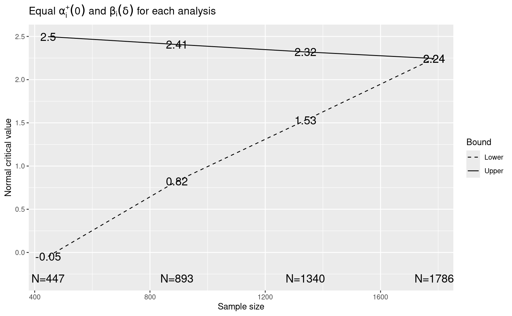
x
#> Asymmetric two-sided group sequential design with
#> 80 % power and 2.5 % Type I Error.
#> Upper bound spending computations assume
#> trial continues if lower bound is crossed.
#>
#>                   ----Lower bounds----  ----Upper bounds-----
#>   Analysis   N    Z   Nominal p Spend+  Z   Nominal p Spend++
#>          1  447 -0.05    0.4816   0.05 2.50    0.0063  0.0063
#>          2  893  0.82    0.7953   0.05 2.41    0.0080  0.0063
#>          3 1340  1.53    0.9370   0.05 2.32    0.0101  0.0063
#>          4 1786  2.24    0.9876   0.05 2.24    0.0124  0.0062
#>      Total                      0.2000                 0.0250
#> + lower bound beta spending (under H1):
#>  Piecewise linear spending function with line points = 0.25, line points = 0.5, line points = 0.75, line points = 0.25, line points = 0.5, line points = 0.75.
#> ++ alpha spending:
#>  Piecewise linear spending function with line points = 0.25, line points = 0.5, line points = 0.75, line points = 0.25, line points = 0.5, line points = 0.75.
#>
#> Boundary crossing probabilities and expected sample size
#> assume any cross stops the trial
#>
#> Upper boundary (power or Type I Error)
#>           Analysis
#>    Theta      1      2      3      4  Total   E{N}
#>   0.0000 0.0063 0.0062 0.0059 0.0042 0.0225  769.7
#>   0.0757 0.1843 0.2805 0.2253 0.1100 0.8000 1054.1
#>
#> Lower boundary (futility or Type II Error)
#>           Analysis
#>    Theta      1      2      3      4  Total
#>   0.0000 0.4816 0.3321 0.1299 0.0339 0.9775
#>   0.0757 0.0500 0.0500 0.0500 0.0500 0.2000
The printed output from the above is shown below and a plot of the derived boundaries is in Figure below. The columns labeled Spend+ and Spend++ show the values \(\beta_i(\delta)\) and \(\alpha_i(0)\), respectively, are equal for each analysis, \(i = 1, 2, 3, 4\). The nominal \(p\)-values for the upper bound increase and thus the bounds themselves decrease for each analysis. That equal error probabilities results in unequal bounds is because of the correlation between the test statistics used for analysis that was indicated in Section 2.1. Note that the requirement of 1372 patients for the fixed design has now increased to a maximum sample size of 1786 which is an inflation of 30%. On the other hand, the expected number of patients when a boundary is crossed is 770 under the assumption of no treatment difference and 1054 under the alternative hypothesis of a 15% event rate in the control group and 10% in the experimental group. Thus, this redesign seems reasonably effective at controlling the sample size when the experimental regimen has no underlying benefit. The nominal \(\alpha-\)level of 0.0124 required for a positive result at the end of the study is almost exactly half that of the overall 0.025 for the study. We will propose other designs that will not require such a small final nominal \(\alpha\) by setting higher early efficacy bounds.
Now we display piecewise linear spending functions. The plot resulting from the code below is displayed below.
# Cumulative proportion of spending planned at each analysis
# Now use a piecewise linear spending
p <- c(0.05, 0.2, 0.5)
p2 <- c(0.6, 0.8, 0.85)
x <- gsDesign(
  k = 4,
  n.fix = n.fix,
  beta = 0.2,
  sfu = sfLinear,
  sfupar = c(t, p),
  sfl = sfLinear,
  sflpar = c(t, p2)
)
plot(x, plottype = "sf", main = "Piecewise linear spending")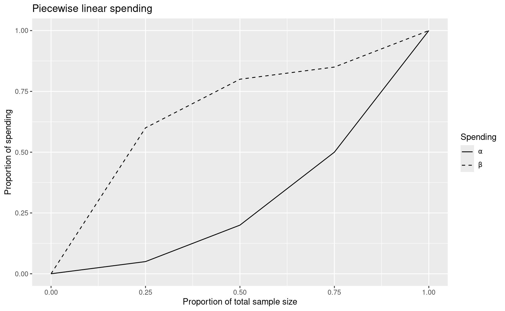
6.2 Deriving group sequential designs using boundary families
The second method of setting boundaries uses the relative \(z\)-value for a design cutoff at each interim analysis, \(c_i>0\), \(i = 1, 2, \ldots, k\). We define vectors \({\bf t}\equiv (t_1, t_2, \ldots, t_k)\) and \({\bf c}\equiv (c_1, c_2, \ldots, c_k)\). For 2-sided testing, Wang and Tsiatis (Wang and Tsiatis 1987) defined the boundary function
\[ -a_i = b_i = C({\bf t},{\bf c}) c_i \]
where the constant \(C({\bf t}, {\bf c})>0\) is chosen to appropriately control Type I error.
Wang and Tsiatis (Wang and Tsiatis 1987) specifically defined the boundary function family
\[ g(t;\Delta)=C({\bf t}; \Delta)t^{\Delta - 0.5}. \]
For \(i = 1, 2, \ldots, k\), the boundary at analysis \(i\) are given by
\[ -a_i = b_i = C({\bf t}; \Delta)t_i^{\Delta - 0.5}. \]
For 2-sided testing, note that for \(\Delta = 0.5\) the boundary values are all equal. Thus, this is equivalent to a Pocock (Pocock 1977) boundary when analyses are equally spaced. The value \(\Delta=0\) generates O’Brien-Fleming bounds (O’Brien and Fleming 1979).
Pampallona and Tsiatis (Pampallona and Tsiatis 1994) derived a related method of using boundary families to set asymmetric bounds; this is not currently implemented in gsDesign(). Using constants \(c^\prime_i>0\), \(i=1, 2, \ldots, k\) and a constant \(C^\prime(\bf t; I_k)\) that along with \(I_k\) is used to appropriately control Type II error, they set
\[ a_i=\delta\sqrt{t_i}-C^\prime({\bf t})c_i^\prime. \]
O’Brien-Fleming, Pocock, or Wang-Tsiatis are normally used with equally-spaced analyses. They are used only with one-sided (test.type=1) and symmetric two-sided (test.type=2) designs. We will use the CAPTURE example, again with 80% power rather than the default of 90%. Notice that this requires specifying beta = 0.2 in both nBinomial() and gsDesign(). O’Brien-Fleming, Pocock, or Wang-Tsiatis (parameter of 0.15) bounds for equally space analyses are generated using the parameters sfu and sfupar below. If you print the Pocock design (xPocock), you will see that the upper bounds are all equal and that the upper boundary crossing values \(\alpha_i(0)\) printed in the Spend column decrease from 0.0091 for the first analysis to 0.0041 for the final analysis.
n.fix <- nBinomial(p1 = 0.15, p2 = 0.1, beta = 0.2)
xOF <- gsDesign(
  k = 4,
  test.type = 2,
  n.fix = n.fix,
  sfu = "OF",
  beta = 0.2
)
xPocock <- gsDesign(
  k = 4,
  test.type = 2,
  n.fix = n.fix,
  sfu = "Pocock",
  beta = 0.2
)
xWT <- gsDesign(
  k = 4,
  test.type = 2,
  n.fix = n.fix,
  sfu = "WT",
  sfupar = 0.15,
  beta = 0.2
)
The resulting sample sizes for these designs can be computed using
We now present an example of how is fairly simple to produce custom plots using gsDesign() output and standard R plotting functions. The resulting output is in Figure below. If you are not familiar with R plotting, executing the following statements one at a time may be instructive. The call help(plot) and its "See also" links (especially par) can be used to find explanations of parameters below. The legend call below particularly demonstrates a nice strength of R for printing Greek characters and subscripts in plots.
plot(
  xOF$n.I,
  xOF$upper$bound,
  xlim = c(300, 1800),
  ylim = c(1.5, 4.5),
  pch = "o",
  cex = 1.5,
  lwd = 2,
  type = "b",
  xlab = "N",
  ylab = "Normal critical value (upper bounds)",
  main = "N and upper bounds with Wang-Tsiatis designs"
)
lines(xPocock$n.I, xPocock$upper$bound, lty = 3, lwd = 2)
points(xPocock$n.I, xPocock$upper$bound, pch = "p", cex = 1.5)
lines(xWT$n.I, xWT$upper$bound, lty = 2, lwd = 2)
points(xWT$n.I, xWT$upper$bound, pch = "x", cex = 1.5)
legend(
  x = c(600, 1825),
  y = c(3.4, 4.5),
  lty = c(1, 2, 3),
  lwd = 2,
  pch = c("o", "x", "p"),
  cex = 1.5,
  legend = c(
    expression(paste(
      Delta, "=0.0, ", N[4],
      "=1404, (O'Brien-Fleming)"
    )),
    c(
      expression(paste(
        Delta, "=0.15, ", N[4], "=1430"
      )),
      c(expression(paste(
        Delta, "=0.50, ", N[4], "=1650, (Pocock)"
      )))
    )
  )
)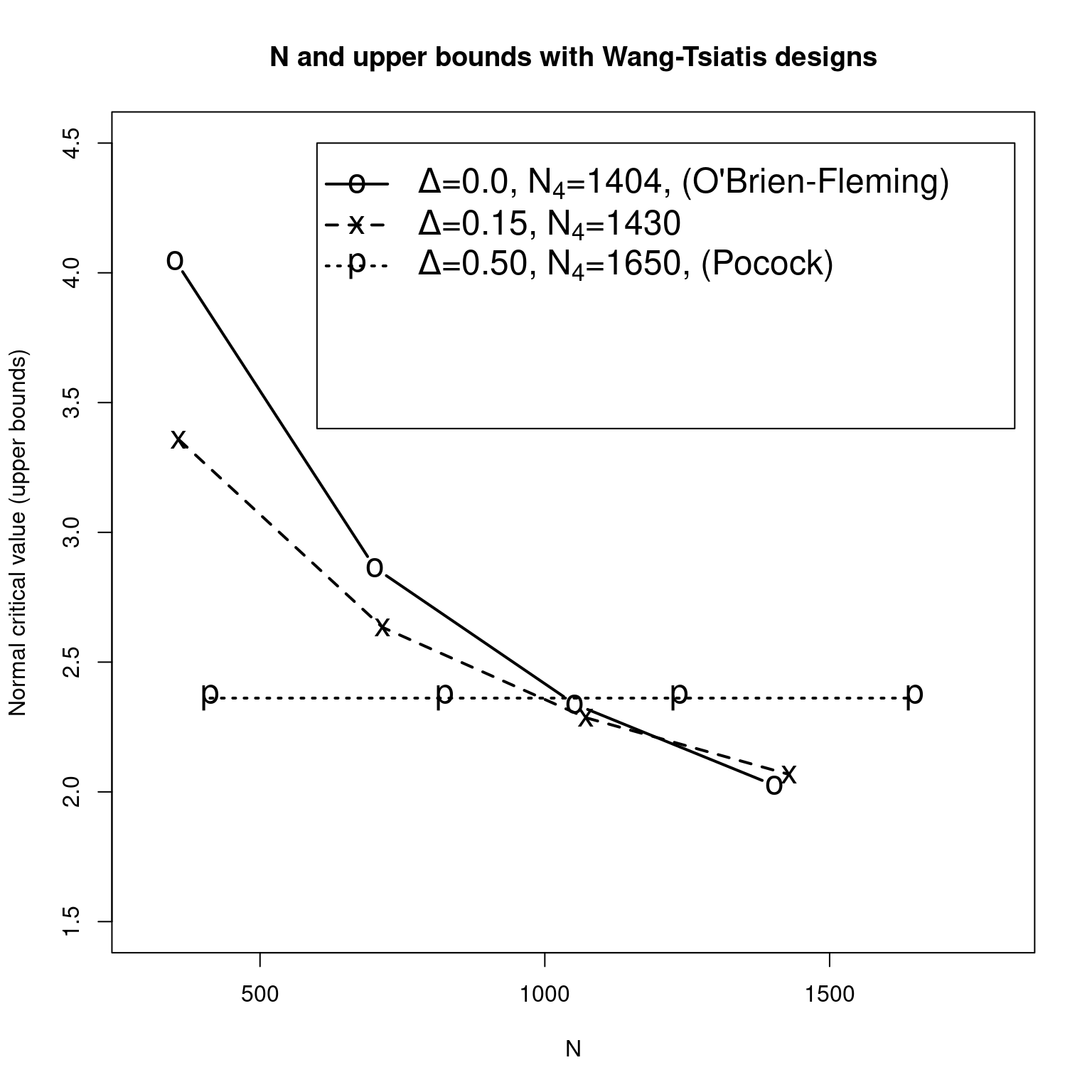
Figure 6.1 shows how the upper bounds and sample size change as \(\Delta\) changes for Wang-Tsiatis bounds. For the O’Brien-Fleming design, the final sample size is only inflated to 1402 from the 1372 required for a fixed design. The relatively aggressive early bounds for the the Pocock design result in sample size inflation to 1650. This design is not frequently used because of the relatively low bounds at early analyses and the substantial sample size inflation required to maintain the desired power. Since the nominal \(p\)-value required for stopping at the initial analysis for the O’Brien-Fleming design is 0.00005 (2-sided), an intermediate design with \(\Delta = 0.15\) might be of some interest. This has a relatively small sample size inflation to 1430 in order to maintain power and the nominal \(p\)-value required to stop the trial at the first interim analysis is \(0.0008\) (2-sided). Examine the boundary crossing probabilities by reviewing, for example, xOF$upper$spend. Also consider reviewing plot(xWT, plottype = 3) to see the observed treatment effect required at each analysis to cross a boundary.