9  Analyzing group sequential trials

We present several ways to review and interpret interim and final results from group sequential trials. Generally, regulatory agencies will have interest in well-controlled Type I error and unbiased treatment estimates.

9.1 The CAPTURE data

We consider interim (Cytel 2007) and final (The CAPTURE Investigators 1997) data from the CAPTURE trial. Table 9.1 provides a summary.

Table 9.1: Summary of the CAPTURE trial.

	Placebo			Experimental
Analysis	Events	n	%	Events	n	%	\(Z\)
1	30	175	17.1%	14	175	8.0%	2.58
2	55	353	15.6%	37	347	10.7%	1.93
3	84	532	15.8%	55	518	10.6%	2.47
4	101	635	15.9%	71	630	11.3%	2.41

The interim data presented here is from finalized datasets rather than the actual data that was analyzed at the time of interim analyses. Also, we take a binomial analysis approach here using the method of Miettinen and Nurminen (Miettinen and Nurminen 1985); the original study analyses used the logrank test. The CAPTURE study was originally designed using symmetric bounds, and the final planned sample size was 1400 patients. The trial was stopped after analyzing the data from 1050 patients. Enrollment continued during follow-up, data entry and cleaning, adjudication and analysis of the data. By the time of the 1050 patient analysis was evaluated and the decision was made to stop the trial, a total of 1265 patients had been enrolled. Following are the data which are then summarized including Z-values using the methods of Miettinen and Nurminen (Miettinen and Nurminen 1985) are used, but without a continuity correction as recommended by Gordon and Watson (Gordon and Watson 1985).

library(gsDesign)

n1 <- c(175, 353, 532, 635)
n2 <- c(175, 347, 518, 630)
x1 <- c(30, 55, 84, 101)
x2 <- c(14, 37, 55, 71)
z <- testBinomial(x1 = x1, x2 = x2, n1 = n1, n2 = n2)
round(z, 2)
#> [1] 2.58 1.93 2.47 2.41

9.2 Testing significance of the CAPTURE data

The Z-statistics computed above can only be interpreted in context of the study design. The original design used a custom spending function which has not been published and will not be discussed further here. Also, while the trial originally had a symmetric, 2-sided design we will use a design with a futility bound here. Below we create an asymmetric design for CAPTURE with a non-binding futility rule and default upper and lower spending functions, but change the upper spending function parameter for the Hwang-Shih-DeCani spending function to \(\gamma=-3\). The original plan was to perform interim analyses after 350 and 700 patients.

The code sequence below is as described follows:

• Compute the fixed design sample size using nBinomial().
• Compute a group sequential design with standard spending functions and interim analyses after 25% and 50% of the data (first call to gsDesign()).
• In order to get timing of interims exactly at 350 and 700 patients, we set the timing of intervals to \(350/n\), \(700/n\) where \(n\) here represents the group sequential design sample size. This required 3 iterations to satisfactorily converge since the required \(n\) changes as the interim timing changes. In the final call to gsDesign() we include the information that the trial is designed to detect a difference in binomial rates and the presumed underlying treatment difference under the alternate hypothesis is 0.05 ($ = 0.15 - 0.10$).
• We then show the sample size and upper bounds at each analysis.
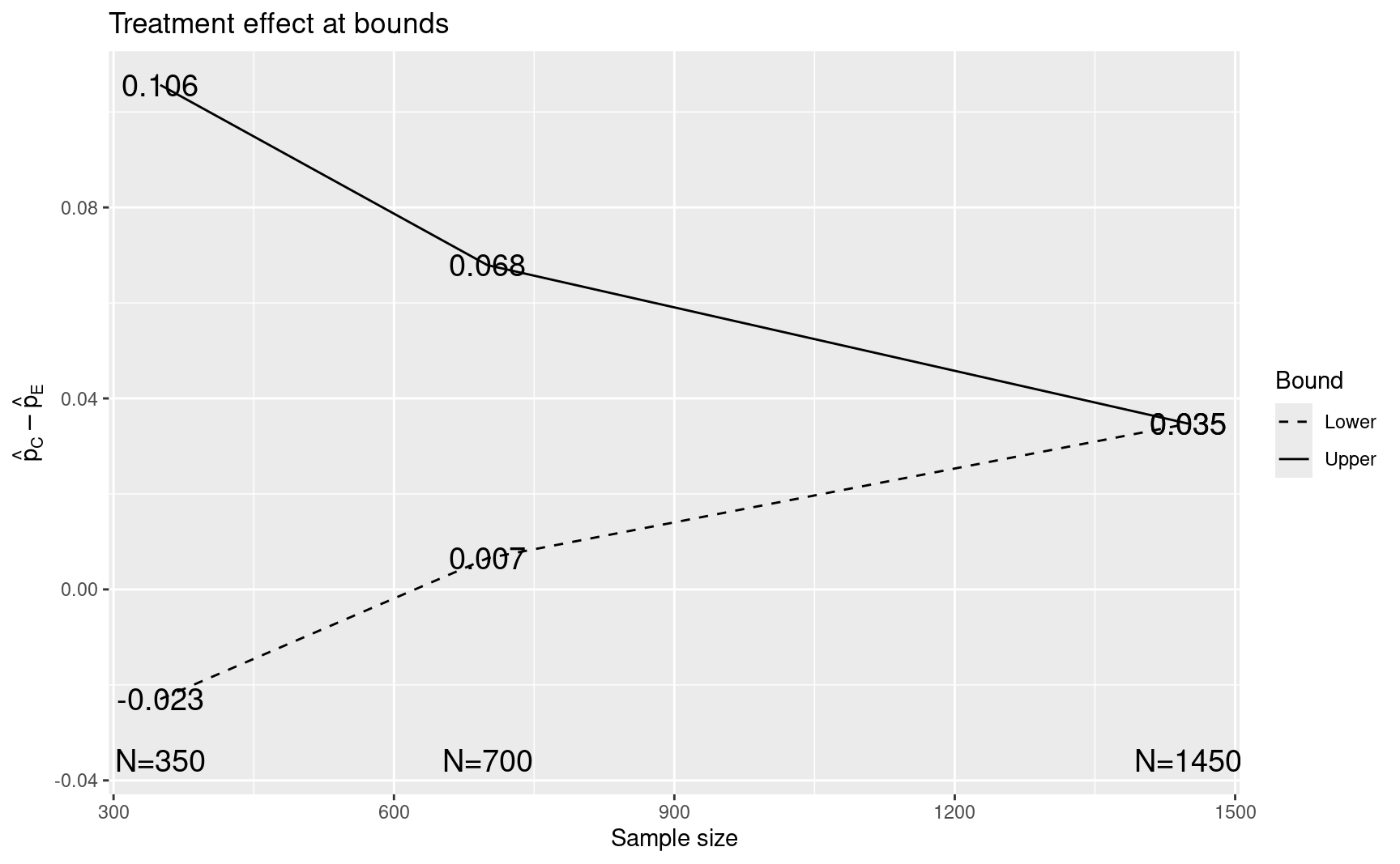
• Finally, we plot the approximate treatment differences required to cross each boundary with 3 digits of accuracy.

n.fix <- nBinomial(p1 = 0.15, p2 = 0.1, beta = 0.2)
x <- gsDesign(
  k = 3,
  n.fix = n.fix,
  beta = 0.2,
  sfupar = -3
)
x <- gsDesign(
  k = 3,
  n.fix = n.fix,
  timing = c(350, 700) / x$n.I[3],
  beta = 0.2,
  sfupar = -3
)
x <- gsDesign(
  k = 3,
  n.fix = n.fix,
  timing = c(350, 700) / x$n.I[3],
  beta = 0.2,
  sfupar = -3
)
CAPTURE <- gsDesign(
  k = 3,
  n.fix = n.fix,
  timing = c(350, 700) / x$n.I[3],
  beta = 0.2,
  sfupar = -3,
  endpoint = "binomial",
  delta1 = 0.05
)
ceiling(x$n.I / 2) * 2
#> [1]  352  702 1452

x$upper$bound
#> [1] 2.990047 2.718060 1.999961

plot(CAPTURE)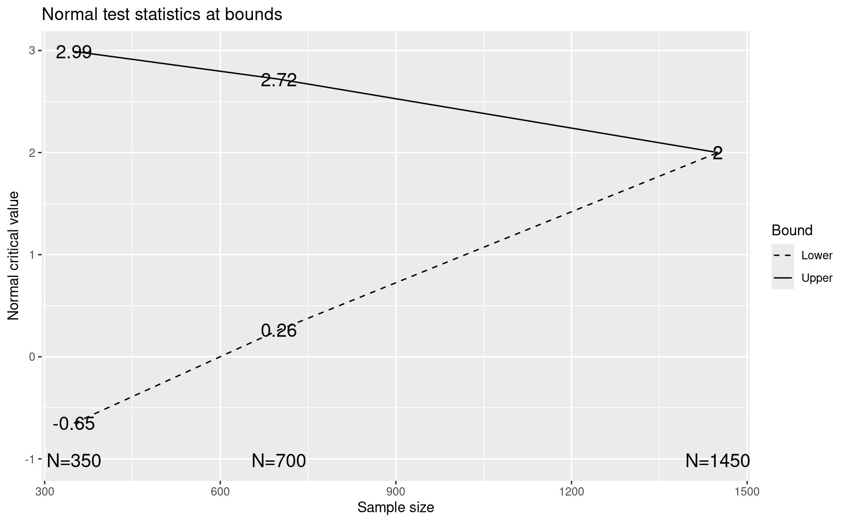

plot(CAPTURE, plottype = "xbar", dgt = c(3, 3))

9.3 Adding an interim analysis to a design

The original design of the CAPTURE trial had two interim analyses planned after 350 and 700 patients. As we have seen, a third interim was added at 1050 patients at the request of the data monitoring committee. The distribution theory for group sequential design requires that timing of interims is independent of interim test statistics. Thus, it would be preferable for a request for an additional interim to come from a group not familiar with the interim unblinded results; in this case, adding the requested interim was discussed with regulators who agreed to building the third interim as if there was no input based on knowledge of unblinded interim results. We will demonstrate how to appropriately control Type I error when an an analysis is added based on unblinded results when discussing conditional power and conditional error later.

The following code demonstrates how to add an interim analysis to a design when interim test statistics are not known. The arguments require are:

• The number of analyses, which is being updated to k = 4.
• The sample size at each analysis in n.I. We keep the originally planned times at 350, 700, and CAPTURE$n.I[3] and add an analysis after 1050 patients.
• The maximum sample size from the original plan in maxn.IPlan.
• The originally planned fixed design sample size in n.fix, original Type II error in beta and original spending function parameters (in this case, defaults plus sfupar).

CAPTURE3IA <- gsDesign(
  k = 4,
  n.I = c(350, 700, 1050, CAPTURE$n.I[3]),
  n.fix = n.fix,
  maxn.IPlan = CAPTURE$n.I[3],
  sfupar = -3,
  beta = 0.2
)
CAPTURE3IA$lower$bound[4]
#> [1] 1.980993

CAPTURE3IA$upper$bound[4]
#> [1] 2.039066

The above adjustment leaves the sample size of the two previously planned interims, the spending functions, and the final analysis sample size alone. This is done by leaving the \(\alpha\)- and \(\beta\)-spending alone at these interims, which is driven by leaving the maximum sample size and spending functions alone. You can see that when a new interim analysis is added to a design without increasing the sample size, the upper and lower boundaries are not the same at the final analysis as they were previously. This is because by adding \(\alpha\)- and \(\beta\)-spending at a third interim analysis, the final boundaries need to be changed to maintain the total \(\alpha\)- and \(\beta\)-spending as desired. Power is measured by the probability of crossing the upper boundary under the alternate hypothesis as stored in sum(CAPTURE3IA$upper$prob[,2]) =0.788. The fact that the upper and lower bounds are not equal to each other means the power to cross the upper bound is somewhat reduced.

To adjust the design, we change the final lower bound to be equal to the upper bound so that Type II error reflects actual decision-making; the final analysis will no longer reflect the originally planned \(\beta\)-spending at the final analysis

cumsum(CAPTURE3IA$lower$spend)
#> [1] 0.01942596 0.05090704 0.10192428 0.20000000

CAPTURE3IA$lower$bound[4] <- CAPTURE3IA$upper$bound[4]
CAPTURE3IA <- gsProbability(
  d = CAPTURE3IA,
  theta = CAPTURE3IA$theta
)
CAPTURE3IA$lower$prob[4, 2]
#> [1] 0.109738

plot(CAPTURE3IA)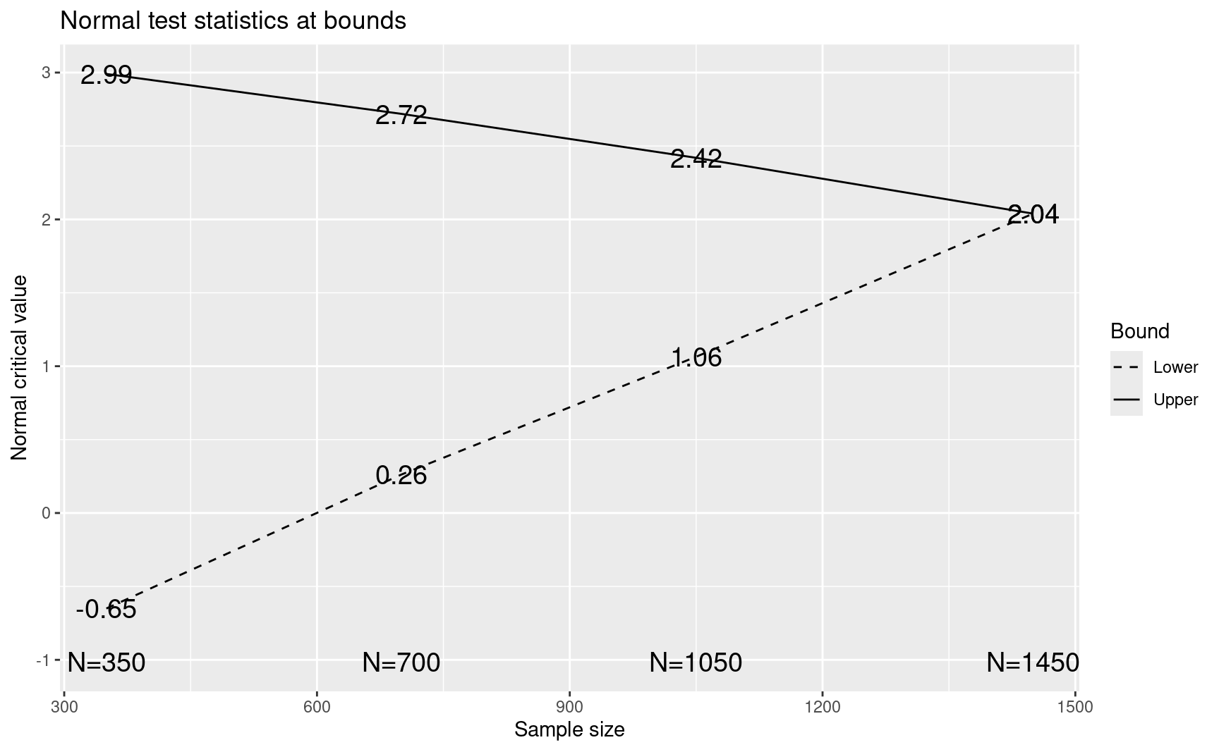

9.4 Stage-wise \(p\)-values

Fairbanks and Madsen (Madsen and Fairbanks 1983) provide a method for computing \(p\)-values for a symmetric group sequential trial design once a boundary has been crossed. Here we will consider just \(p\)-values for positive efficacy findings for asymmetric designs. We assume for some \(i\) in \(1, 2, \ldots, k\) that an upper bound is first crossed at analysis \(i\) with a test statistic values \(z_i\). The stage-wise \(p\)-value uses the same computational method as \(\alpha^+(0)\) from equation

\[ \alpha^+(\theta) \equiv\sum_{i=1}^{k}\alpha^+_{i}(\theta) \]

\[ p_{SW}=P_{0}\{\{Z_{i}\geq z_{i}\}\cap_{j=1}^{i-1}% \{Z_{j}<b_{j}\}\} \]

This formula can still be used for the final analysis when the upper bound is never crossed. This method of computing \(p\)-values emphasizes early positive results and de-emphasizes late results. No matter how positive a result is after the first analysis, the \(p\)-value associated with a positive result will not be smaller than a first analysis result that barely crosses its bound. There is no way to compute a \(p\)-value if, for some reason, you stop a trial early without crossing a bound. For the CAPTURE data analyzed according to the default design derived above, we compute a stagewise \(p\)-value by replacing the upper boundary at the third interim analysis with the \(Z\)-value that crossed that bound. The stagewise \(p\)-value is then the probability of crossing an upper bound at the first 3 interim analyses assuming this modified bound.

b <- CAPTURE3IA$upper$bound[1:2]
b <- c(b, z[3])
y <- gsProbability(
  k = 3,
  theta = 0,
  n.I = CAPTURE3IA$n.I[1:3],
  a = array(-20, 3),
  b = b
)
sum(y$upper$prob)
#> [1] 0.009259521

9.5 Repeated confidence intervals

Repeated confidence intervals use the nominal Type I error at each interim analysis to compute confidence bounds in the usual fashion. For the binomial analysis of the CAPTURE trial we use Miettinen and Nurminen (Miettinen and Nurminen 1985) confidence intervals at 2 times the nominal \(\alpha\)-level of the upper bound, \(2\times(1-\Phi(u_k))\), \(i=1,2,\ldots,k\).

gsBinomialRCI <- function(d, x1, x2, n1, n2) {
  y <- NULL
  rname <- NULL
  nanal <- length(x1)
  for (i in 1:nanal) {
    y <- c(y, ciBinomial(
      x1 = x1[i], x2 = x2[i], n1 = n1[i],
      n2 = n2[i], alpha = 2 * pnorm(-d$upper$bound[i])
    ))
    rname <- c(rname, paste("Analysis", i))
  }
  ci <- matrix(y, nrow = nanal, ncol = 2, byrow = T)
  rownames(ci) <- rname
  colnames(ci) <- c("Lower CI", "Upper CI")
  ci
}
rci <- gsBinomialRCI(
  CAPTURE3IA,
  x1[1:3],
  x2[1:3],
  n1[1:3],
  n2[1:3]
)
pdif <- (x1 / n1 - x2 / n2)[1:3]
pdif
#> [1] 0.09142857 0.04917912 0.05171713

rci
#>            Lower CI    Upper CI 
#> Analysis 1 -0.01554062 0.2032692
#> Analysis 2 -0.02080474 0.1200844
#> Analysis 3 0.001147321 0.102811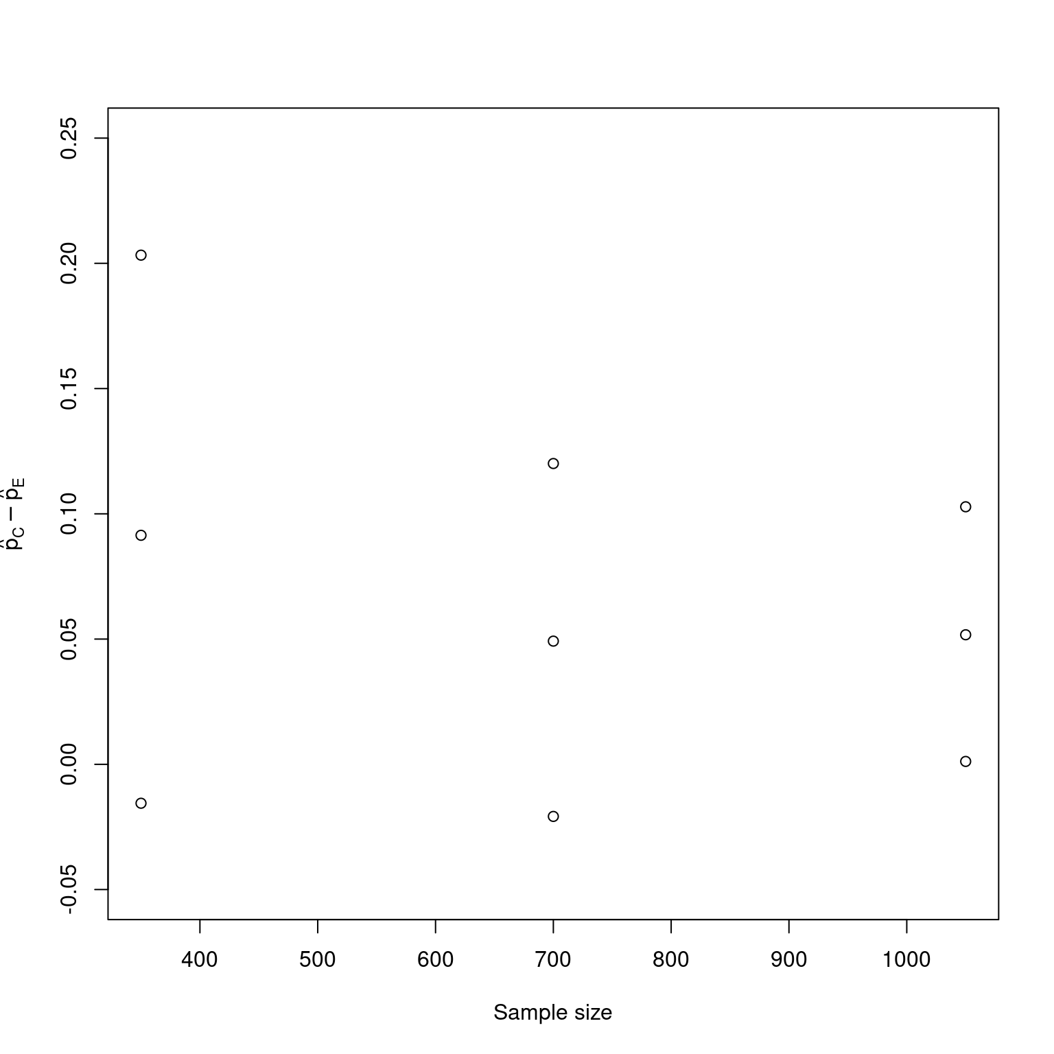

plot((n1 + n2)[1:3], rci[, 2],
  ylim = c(-0.05, 0.25), xlab = "Sample size",
  ylab = expression(hat(p)[C] - hat(p)[E])
)
points((n1 + n2)[1:3], rci[, 1])
points((n1 + n2)[1:3], pdif)

Figure 9.1

9.6 Subdensity functions

The subdensity functions defined here are useful for purposes of estimation as discussed by Jennison and Turnbull (Jennison and Turnbull 2000), Chapter 8. In particular, these may be used for stagewise confidence intervals. We define a subdensity function for the probability that a trial continues without crossing a boundary until analysis \(i\), and then the \(Z\)-value takes on a value \(z\) at that analysis, \(i=1,2,\ldots,k\):

\[ p_i(z|\theta)=\frac{d}{dz}P_{\theta}\{\{Z_{i}\geq z\}\cap_{j=1}^{i-1} \{ l_{j}<Z_{j}< u_{j}\}\}, \tag{9.1}\]

These subdensity functions are used to compute \(\alpha_i(\theta)\) as defined in equation

\[ \alpha_{i}(\theta)=P_{\theta}\{\{Z_{i}\geq u_{i}\}\cap_{j=1}^{i-1} \{ l_{j}<Z_{j}< u_{j}\}\}, i = 1, 2, \ldots, k. \]

Normally, this will not be of great concern to the reader even though this computation will go on “behind the scenes” each time a group sequential design is derived or boundary crossing probability computed. However, a subdensity function for a design may be computed using the function gsDensity() as follows. In ?fig-gsdensity, we replicate parts of Figure 8.1 and Figure 8.2 of Jennison and Turnbull ((Jennison and Turnbull 2000)) which show the subdensities for an O’Brien-Fleming design with four analyses.

We will later apply Equation 9.1 to compute a posterior distribution for \(\theta\) given an interim test statistic \(Z_i=z\) at analysis, \(i\), \(1\leq i \leq k\).

Cytel, Inc. 2007. EAST 5. Cambridge, MA: Cytel, Inc.

Gordon, Ian, and Ray Watson. 1985. “The Myth of Continuity-Corrected Sample Size Formulae.” Biometrics 52 (1): 71–76.

Jennison, Christopher, and Bruce W. Turnbull. 2000. Group Sequential Methods with Applications to Clinical Trials. Boca Raton, FL: Chapman; Hall/CRC.

Madsen, Richard W, and Kenneth B Fairbanks. 1983. “\(P\) Values for Multistage and Sequential Tests.” Technometrics 25 (3): 285–93.

Miettinen, Ollie, and Markku Nurminen. 1985. “Comparative Analysis of Two Rates.” Statistics in Medicine 4 (2): 213–26.

The CAPTURE Investigators. 1997. “Randomised Placebo-Controlled Trial of Abciximab Before and During Coronary Intervention in Refractory Unstable Angina: The CAPTURE Study.” The Lancet 349 (9063): 1429–35.