11  Bayesian design properties

All of the properties of group sequential designs we have considered so far have depended on knowing an exact value \(\theta\) measuring treatment effect. Some evaluations may benefit from taking into account uncertainty concerning \(\theta\). Rather than assuming a fixed value of \(\theta\) to compute quantities such as power, Type I error and expected sample size, we consider these quantities based on a prior distribution for \(\theta\). Power and Type I error are replaced by probability of success when averaging over a prior distribution. By assigning a value to a trial outcome, the prior distribution for \(\theta\) can be used to compute the value of a trial design. Given built-in optimization functions in R, it is then easy to apply gsDesign functions to optimize specific characteristics of a trial design such as a futility bound or spending function.

After an interim result, we can again update the uncertainty about \(\theta\) by computing a posterior distribution. Conditional power can be replaced by predictive power by averaging conditional power over this posterior distribution. The value of the trial can be replaced by the predictive value which conditions on an interim outcome. We can also compute prediction intervals for future trial results conditioned on an interim outcome. All of these measures can be based on a specific interim result or (blinded) knowledge that no trial boundary has been crossed. The latter may be particularly useful for a sponsor to update their internal estimates for the ultimate probability that a trial is successful.

In summary, the following questions may be answered using a Bayesian approach:

• What is the probability of success of the trial?
• Based on a specified utility function, what is the value of a trial design?
• What is the posterior for \(\theta\) given an interim result?
• What is the predictive distribution of future observations given an interim result?
  • What is the predictive probability of success?
  • Can we compute prediction intervals for future results?
  • What is the value of a trial conditional on the interim result?

Examples in this section compute answers to all of these questions when framed in terms of a particular trial.

11.1 Normal densities

The primary tool for computing group sequential probabilities is application of numerical integration of a normal density function. The normalGrid() function is a lower-level function used by gsProbability() and gsDesign() that is normally obscured from the user. For Bayesian computations with a normal prior distribution, such as here, it can be quite useful. Since this also has many potential applications in areas - not restricted to group sequential design - we have made this function available to users. The reason for making a separate function rather than just using the R function pnorm() is that normalGrid() computes grid weights for numerical integration using Simpon’s method as recommended by Jennison and Turnbull in Chapter 19 (Jennison and Turnbull 2000). Figure 11.1 shows a plot of weights for numerical integration from a standard normal distribution as generated below. We can integrate out the expected value of a function of a standard normal distribution by multiplying the value of the function at each point on the grid by the grid weights and summing to integrate. This is illustrated by computing the \(E\{Z^2\}=1\) below. The density evaluated at values in g$z are stored in g$density, if needed.

library(gsDesign)

g <- normalGrid(mu = 0, sigma = 1)
sum(g$z^2 * g$wgts)
#> [1] 1.000001

plot(g$z, g$wgts)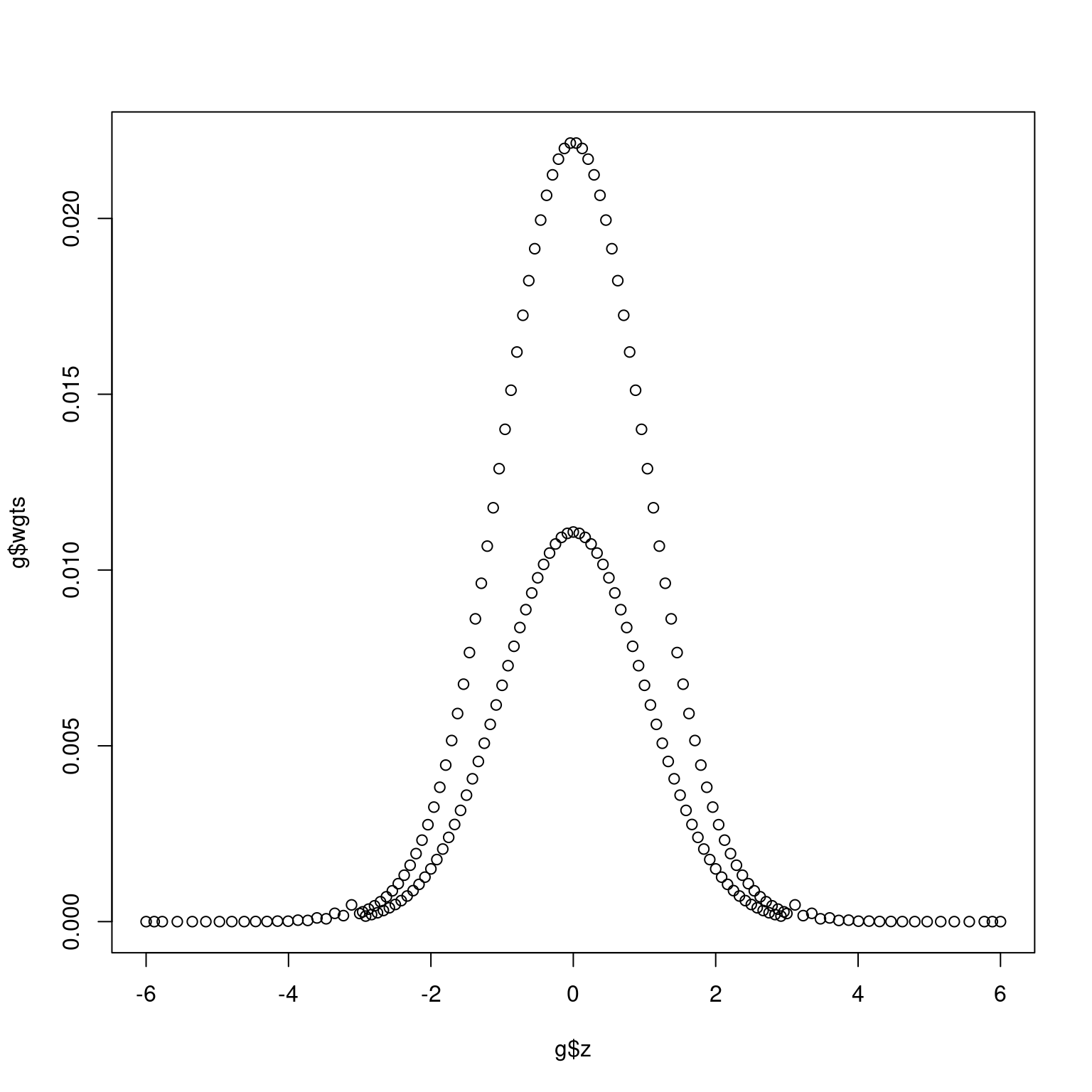

Figure 11.1: Weights for numerical integration from a standard normal distribution.

We demonstrate the use of normalGrid() to generate a prior distribution for the parameter of interest in a group sequential design below. This will then be used in various Bayesian applications in later sections. Here we simply describe the use of the normalGrid() function used to work with normal densities.

Next we plot normal densities with mean 0 and 0.5 and standard deviations 1 and 2, respectively, in Figure 11.2 and Figure 11.3.

g <- normalGrid(mu = 0, sigma = 1)
plot(g$z, g$wgts, main = "mean=0, standard deviations=1")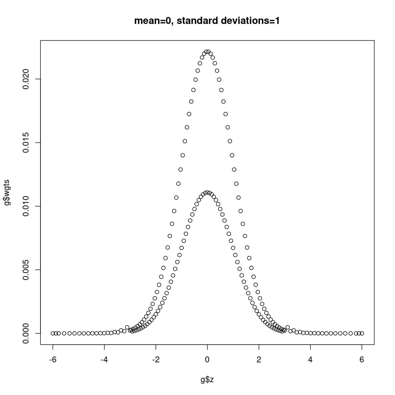

Figure 11.2

g <- normalGrid(mu = 0.5, sigma = 2)
plot(g$z, g$wgts, main = "mean=0.5, standard deviations=2")

Figure 11.3

We then add a normal density with range -5 to -2 with mean -4 and standard deviation 1.5 in Figure 11.4.

d1 <- normalGrid()
d2 <- normalGrid(mu = 0.5, sigma = 2)
minx <- min(d1$z, d2$z)
maxx <- max(d1$z, d2$z)
plot(
  x = d2$z,
  y = d2$density,
  type = "l",
  xlim = c(minx, maxx),
  ylim = c(0, max(d1$density)),
  xlab = "z",
  ylab = "Density",
  lwd = 2,
  main = "Normal density examples."
)
lines(x = d1$z, y = d1$density, lty = 2, lwd = 2)
d3 <- normalGrid(mu = -4, sigma = 1.5, bounds = c(-5, -2))
lines(x = d3$z, y = d3$density, lwd = 2, lty = 3)
legend(
  x = c(4, 7),
  y = c(0.27, 0.4),
  lty = c(2, 1, 3),
  lwd = 2,
  legend = c("d1", "d2", "d3")
)

Figure 11.4

11.2 The posterior distribution for \(\theta\)

For a given parameter sample space of real-values \(\Theta\), denote the prior distribution function for \(\theta\in\Theta\) at the beginning of the trial by \(G(\theta)\). This may represent a continuous or discrete distribution or a combination of the two. The joint sub-density of \(\theta\), the interim test statistics not crossing a bound prior to analysis \(i\), and an interim value \(z\) at analysis \(i\), \(1\leq i\leq k\) is

\[ p_i(z|\theta)\frac{d}{d\theta}G(\theta). \]

To obtain a posterior distribution, we integrate over all possible values of \(\theta\in\Theta\) to get a marginal density for \(Z_i=z\) at analysis \(i\) for the denominator in the following equation for the posterior distribution of \(\theta\) given no boundary crossing prior to analysis \(i\) and the interim test statistic \(Z_i=z\), \(1\leq i\leq k\):

\[ dG_i(\theta|z)=\frac{p_i(z|\theta)dG(\theta)/d\theta} {\int_{\eta\in\Theta} p_i(z|\eta)dG(\eta)/d\eta G_i(z,\eta)}. \tag{11.1}\]

When a sufficient statistic \(\hat{\theta}\) is available to estimate \(\theta\) at an interim analysis, the marginal distribution can be factored into the joint distribution of the sufficient statistic \(\hat{\theta}\) and \(\theta\) times a function of the individual data points that is independent of \(\theta\). This means computing the posterior distribution can ignore the individual data points. Proschan, Lan and Wittes (Proschan, Lan, and Wittes 2006) show the posterior distribution under the assumption of a normal prior. Their formulation is that \(\theta=E\{Z_k\}\), where \(Z_k\) is the test statistic at the final planned analysis. The formulation here has \(\sqrt{n_k}\theta=E\{Z_k\}\), and we translate the Proschan, Lan and Wittes formulation appropriately. Assuming the prior distribution

\[ \theta\sim N(\theta_0,\sigma_0^2) \]

the posterior distribution conditioning on an interim test statistic \(z_i\) (or \(B_i=b=z_i\sqrt{t_i}\)) at interim \(i\) for \(1\leq i\leq k\) is normal with mean

\[ E\{\theta|Z_i=z_i\}=\frac{\theta_0/\sigma_0^2 + \sqrt{n_i} z_i}{ 1/\sigma_0^2 +n_i} =\frac{\theta_0/\sigma_0^2 + \sqrt{n_k} b}{1/\sigma_0^2 +n_i} \tag{11.2}\]

and variance

\[ \hbox{Var}\{\theta|Z_i=z_i\}=(1/\sigma_0^2+n_i)^{-1}. \tag{11.3}\]

Note that the conditional variance does not depend on \(z_i\). The value \(E\{\theta|Z_i=z_i\}\) is a weighted average of the prior mean and an estimate of \(\theta\) based on data. The weights are the statistical information (inverse of the variance) for each estimate. The total statistical information for the combined estimate (inverse of the posterior variance) is the sum of the statistical information for each estimate.

To demonstrate the above calculation, we again consider the CAPTURE study and assume a normal prior distribution for \(\theta\) with a mean of \(.4\theta_1\) where \(\theta_1\) is the alternate hypothesis value of \(\theta\) and an uninformative standard deviation of \(6\theta_1\). Code to generate this prior using normalGrid() is as follows:

n.fix <- nBinomial(p1 = 0.15, p2 = 0.1, beta = 0.2)
x <- gsDesign(
  k = 3,
  n.fix = n.fix,
  beta = 0.2,
  sfupar = -3
)
x <- gsDesign(
  k = 3,
  n.fix = n.fix,
  timing = c(350, 700) / x$n.I[3],
  beta = 0.2,
  sfupar = -3
)
x <- gsDesign(
  k = 3,
  n.fix = n.fix,
  timing = c(350, 700) / x$n.I[3],
  beta = 0.2,
  sfupar = -3
)
CAPTURE <- gsDesign(
  k = 3,
  n.fix = n.fix,
  timing = c(350, 700) / x$n.I[3],
  beta = 0.2,
  sfupar = -3,
  endpoint = "binomial",
  delta1 = 0.05
)

CAPTURE$delta
#> [1] 0.07565793

sigma1sq <- 6 * CAPTURE$delta^2
mu <- 0.4 * CAPTURE$delta
prior <- normalGrid(mu = mu, sigma = sqrt(sigma1sq))

Next we compute the posterior distribution and, following each analysis, the posterior density. We then see the posterior probability that \(\theta \leq 0\) a priori and after each analysis and compare this to the nominal \(p\)-value for each z-statistic. The prior we have used is relatively uninformative, so the \(p\)-values and posterior probabilities are quite similar. The slight favorable prior lowers the posterior probability compared to nominal \(p\)-values. The interim data and statistics are as we have computed them in Chapter 9.

n1 <- c(175, 353, 532, 635)
n2 <- c(175, 347, 518, 630)
x1 <- c(30, 55, 84, 101)
x2 <- c(14, 37, 55, 71)
z <- testBinomial(x1 = x1, x2 = x2, n1 = n1, n2 = n2)

n <- n1 + n2
postmean <- (mu / sigma1sq + z * sqrt(n)) / (1 / sigma1sq + n)
postvar <- 1 / (1 / sigma1sq + n)
round(postmean, 3)
#> [1] 0.130 0.071 0.075 0.067

round(sqrt(postvar), 3)
#> [1] 0.051 0.037 0.030 0.028

round(pnorm(-c(mu, postmean) / sqrt(c(sigma1sq, postvar))), 4)
#> [1] 0.4351 0.0058 0.0275 0.0068 0.0081

round(1 - pnorm(z), 4)
#> [1] 0.0049 0.0271 0.0067 0.0081

Next we compute the posterior density for \(\theta\) at each analysis using Equation 11.2 and Equation 11.3.

post1den <- normalGrid(mu = postmean[1], sigma = sqrt(postvar[1]))
post2den <- normalGrid(mu = postmean[2], sigma = sqrt(postvar[2]))
post3den <- normalGrid(mu = postmean[3], sigma = sqrt(postvar[3]))
post4den <- normalGrid(mu = postmean[4], sigma = sqrt(postvar[4]))

In order to do a check, we could have also computed the posterior after the first interim analysis with

post2 <- gsPosterior(x = CAPTURE, i = 2, zi = z[2], prior = prior)

If \(z\) represents a set of values (e.g., an interval) and \(p_i(z|\theta)\) the probability that \(Z_i \in z\) given \(\theta\), then we can still apply the equation posterior. The likelihood is computed for not crossing a bound prior to analysis i and being in the interval specified in the 2-values specified in zi. The default if zi is not given is to use the interval between the upper an lower bound at the analysis specified in i, as in the following example. We compute such posterior distributions for the first 3 analyses.

CAPTURE3IA <- gsDesign(
  k = 4,
  n.I = c(350, 700, 1050, CAPTURE$n.I[3]),
  n.fix = n.fix,
  maxn.IPlan = CAPTURE$n.I[3],
  sfupar = -3,
  beta = 0.2
)

post1b <- gsPosterior(x = CAPTURE3IA, i = 1, prior = prior)
post2b <- gsPosterior(x = CAPTURE3IA, i = 2, prior = prior)
post3b <- gsPosterior(x = CAPTURE3IA, i = 3, prior = prior)

Finally, we plot the prior and posteriors where the interim statistics are known in black as well as the posteriors when it is only known that a boundary has not been crossed in red. Since there is less information in the latter, red posteriors, they are more disperse than the corresponding posterior when the interim test statistic is known. The central location for the latter posteriors is also closer to the original prior than the posteriors based on exact results where the posteriors more shift to match the data.

plot(
  post4den$z, post4den$density,
  type = "l", lty = 5,
  xlab = expression(theta), ylab = "Density"
)
lines(post3den$z, post3den$density, lty = 4)
lines(post2den$z, post2den$density, lty = 3)
lines(post1den$z, post1den$density, lty = 2)
lines(prior$z, prior$density)
legend(
  x = c(-0.1, -0.03), y = c(6, 14), lty = c(1:5), lwd = 2,
  legend = c(
    "Prior", "Analysis 1", "Analysis 2", "Analysis 3", "Analysis 4"
  )
)
lines(post1b$z, post1b$density, lty = 2, col = 2)
lines(post2b$z, post2b$density, lty = 3, col = 2)
lines(post3b$z, post3b$density, lty = 4, col = 2)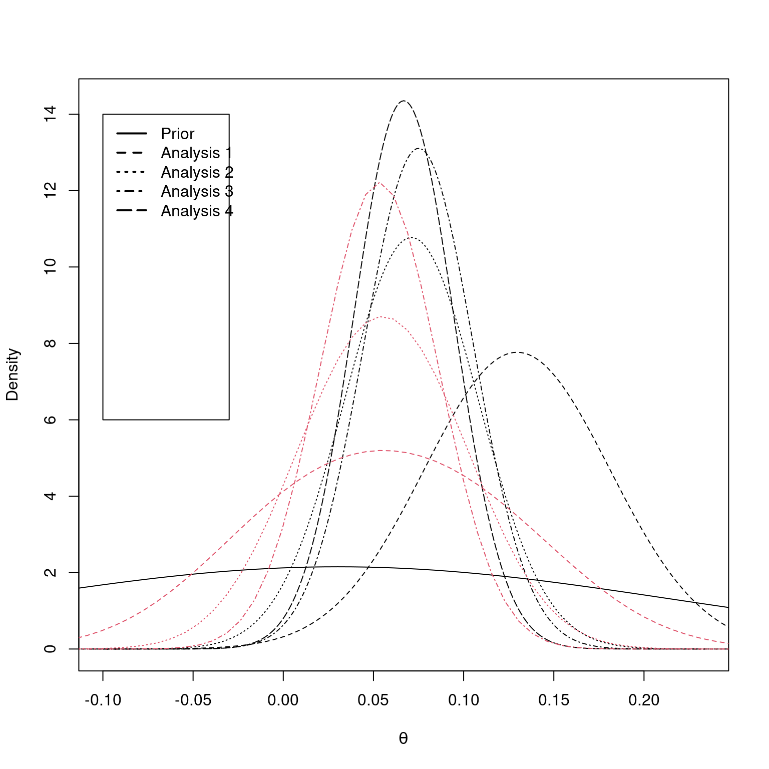

Figure 11.5

11.3 Bayes credible intervals

A Bayes credible interval can be computed using the posterior distribution for \(\theta\). Let \(G_i^{-1}(\cdot |Z_i=z_i)\) be the inverse of \(G_i(\cdot |Z_i=z_i)\). For an interval at level \(1-\alpha/2\), the Bayes credible interval for \(\theta\) given \(Z_i=z_i\) is \((G_i^{-1}(\alpha/2 |Z_i=z_i), G_i^{-1}(1-\alpha/2 |Z_i=z_i)\). We continue the example with a normal prior and posterior. The Bayes credible interval is simply quantiles from a normal distribution with parameters Equation 11.2 and Equation 11.3. Extending our previous example, this can be computed for each analysis of CAPTURE using the inverse standard normal function qnorm() as follows

lCredInt <- postmean + qnorm(0.025) * sqrt(postvar)
uCredInt <- postmean + qnorm(0.975) * sqrt(postvar)
CredInt <- as.matrix(cbind(lCredInt, postmean, uCredInt))
rownames(CredInt) <- paste("Analysis", 1:4)
colnames(CredInt) <- c("Lower", "Mean", "Upper")
CredInt
#>                   Lower       Mean     Upper
#> Analysis 1  0.028963082 0.12962419 0.2302853
#> Analysis 2 -0.001507327 0.07107813 0.1436636
#> Analysis 3  0.015387474 0.07505169 0.1347159
#> Analysis 4  0.012299533 0.06678258 0.1212656

11.4 Predictive power

The credible intervals for \(\theta\) are fairly wide, suggesting that computing conditional power based on a fixed value of \(\theta\) may be misleading. Predictive power extends the concept of conditional power by incorporating uncertainty about the parameter \(\theta\) into computations. Recall that we have denoted the conditional probability of crossing an efficacy boundary at analysis \(j\) given an interim test statistic \(z_i\) at analysis \(i<j\) and parameter \(\theta\) as \(\alpha_{i,j}(\theta|z_i)\). Given a posterior distribution \(G_i(\theta|z_i)\) for \(\theta\) after observing an interim test statistic \(z_i\) defined on some set of values \(\Theta\), the predictive probability of crossing the efficacy boundary at analysis \(j>i\) is defined in Equation 11.4.

\[ \alpha_{i,j}(z_i, G_i)=\int_\Theta \alpha_{i,j}(\theta|z_i)dG_i(\theta|z_i). \tag{11.4}\]

Predictive probability is computed using the function gsPP() as demonstrated below. The first line computes the predictive power to cross a bound at any future analysis. The second line, by specifying total=FALSE, computes the predictive power of crossing a bound at the individual future planned analyses.

gsPP(
  x = CAPTURE,
  zi = z[1],
  i = 1,
  theta = prior$z,
  wgts = prior$wgts
)
#> [1] 0.9633891

gsPP(
  x = CAPTURE,
  zi = z[1],
  i = 1,
  theta = prior$z,
  wgts = prior$wgts,
  total = FALSE
)
#>           [,1]
#> [1,] 0.7984714
#> [2,] 0.1649177

11.5 Predictive distribution for the normal case

For \(1\leq i< j\leq K\), the simple conditional distribution for \(B_j\) given \(B_i=b\) is easily extended to a predictive distribution when the prior for \(\theta\) is normally distributed. Given \(B_i=b\), we consider that

\[ B_j=b+B_{i,j}=b+(t_j-t_i)\sqrt{n_k}\theta+(B_{i,j}-(t_j-t_i)\sqrt{n_k}\theta). \]

Conditioning on \(\theta\), \(B_{i,j}-(t_j-t_i)\sqrt{n_k}\theta\sim N(0,t_j-t_i)\) and because this does not depend on \(\theta\) it has the same unconditional distribution. We know the posterior distribution for \(\theta\) given \(B_i=b\) is normal with mean from Equation 11.2 and variance from Equation 11.3. Thus, we derive that the predictive distribution for \(B_j\) given \(B_i=b\) is normal with

\[ E\{B_j|B_i=b\}=b+E\{B_{i,j}\} =b+\sqrt{n_k}(t_j-t_i)E\{\theta|B_i=b\} \tag{11.5}\]

and

\[ \hbox{Var}\{B_{j}|B_i=b\}=(t_j-t_i)\left(1+\frac{n_k(t_j-t_i)}{1/\sigma_0^2+n_i} \right) \tag{11.6}\]

We now the compute predictive probability of a positive trial at the second interim analysis of the CAPTURE trial using this posterior distribution and compare to gsPP(). Recall that we have already computed the posterior mean and variance for \(\theta\) at each analysis in postmean and postvar, respectively, and the proportion of final planned statistical information at the planned analyses in ti.

gsPP(
  x = CAPTURE,
  zi = z[2],
  i = 2,
  theta = prior$z,
  wgts = prior$wgts
)
#> [1] 0.7643489

ti <- c((n1 + n2)[1:2] / CAPTURE$n.I[3], 1)

b <- z[2] * sqrt(ti[2])
pimean <- b + postmean[2] * (ti[3] - ti[2]) * sqrt(CAPTURE$n.I[3])
pivar <- (postvar[2] + 1) * (ti[3] - ti[2])
pivar <- (postvar[2] * (CAPTURE$n.I[3] - 700) + 1) * (ti[3] - ti[2])
bfinal <- CAPTURE$upper$bound[3]
pnorm(bfinal, mean = pimean, sd = sqrt(pivar), lower.tail = FALSE)
#> [1] 0.764337

The predictive probability for a positive final outcome is slightly below the originally planned power of 80%, but probably not sufficient amount to raise substantial concern.

11.6 Prediction intervals

Prediction intervals for a future test statistic or final treatment effect can be computed using the inverse of the predictive distribution for \(B_j\) given \(B_i\), \(1\leq i<j\leq K\). We continue the above normal distribution example using Equation 11.5 and Equation 11.6. We will ignore intervening interim analysis decisions in this computation, which conditions on the results at the first interim and computes a 90% prediction interval. The inverse normal distribution qnorm() is applied as for the Bayes credible interval computation in Section 11.3.

bpi <- pimean + qnorm(c(0.05, 0.95)) * sqrt(pivar)
bpi
#> [1] 1.052884 4.422583

While the above computation is useful given a normal prior, we also have the gsPI() function to produce a prediction interval for any future analysis given an interim result. Note that the prediction for future analyses again ignores any intervening interim boundaries. The argument i is the interim we condition on, while zi is the test statistic at that analysis. The analysis we are predicting for is indicated by j, and the group sequential design by x. We first reproduce the interval above and then examine prediction intervals for the second and final analyses based on the first interim. Finally, the default level = 0.95 produces a 95% prediction interval. By specifying level = 0 we get a point estimate of the predicted outcome for the second interim analysis based on the first interim. While the second interim \(Z\)-value falls well within the prediction interval based on the first interim, it is quite different than the predicted outcome. Thus, the prediction interval suggests the differences between first and second analysis trends are consistent with variability early in the study.

gsPI(
  level = 0.9,
  x = CAPTURE,
  i = 2,
  j = 3,
  zi = z[2],
  theta = prior$z,
  wgts = prior$wgts
)
#> [1] 1.052837 4.422774

gsPI(
  level = 0.9,
  x = CAPTURE,
  i = 1,
  j = 2,
  zi = z[1],
  theta = prior$z,
  wgts = prior$wgts
)
#> [1] 1.925884 5.151808

gsPI(
  level = 0.9,
  x = CAPTURE,
  i = 1,
  j = 3,
  zi = z[1],
  theta = prior$z,
  wgts = prior$wgts
)
#> [1] 2.182131 7.841837

gsPI(
  level = 0,
  x = CAPTURE,
  i = 1,
  j = 2,
  zi = z[1],
  theta = prior$z,
  wgts = prior$wgts
)
#> [1] 3.538895

z[2]
#> [1] 1.925467

The prediction interval for the standardized treatment effect \(\theta\) divides the above interval by \(\sqrt{n_3}\). Since the analysis we are predicting for is the final analysis, \(b_3=t_3z_3=z_3\) and the prediction intervals are identical.

zpi <- bpi / sqrt(ti[3])
thetapi <- zpi / sqrt(CAPTURE$n.I[3])
zpi
#> [1] 1.052884 4.422583

thetapi
#> [1] 0.0276506 0.1161449

The prediction interval is quite wide which is perhaps counterintuitive given the the predictive probability 0.764 from the previous section.

11.7 Probability of success

The probability of a positive trial depends on the distribution of outcomes in the control and experimental groups. The probability of a positive trial given a particular parameter value \(\theta\) was defined in

\[ \alpha_{i}(\theta)=P_{\theta}\{\{Z_{i}\geq u_{i}\}\cap_{j=1}^{i-1} \{ l_{j}<Z_{j}< u_{j}\}\}, i = 1, 2, \ldots, k. \]

and

\[ \alpha(\theta)\equiv\sum_{i=1}^{k}\alpha_{i}(\theta). \]

as

\[ \alpha(\theta)=\sum_{i=1}^{K} P_{\theta}\{\{Z_{i}\geq b_{i}\}\cap_{j=1}^{i-1} \{a_{j}<Z_{j}<b_{j}\}\}. \]

If we consider \(\theta\) to have a given prior distribution at the beginning of the trial, we can compute an unconditional probability of success for the trial. In essence, since we do not know if the experimental treatment works better than control treatment, we assign some prior beliefs about the likelihood that experimental is better than control and use those along with the size of the trial to compute the probability of success. The prior distribution for \(\theta\) can be discrete or continuous. If the distribution is discrete, we define \(m+1\) values \(\theta_0<\theta_2\ldots<\theta_m\) and assign prior probabilities \(P\{\theta=\theta_j\}\), \(0\leq j\leq m\) such that \(\sum_{j=1}^m P\{\theta_j\}=1\). The probability of success for the trial is then defined as

\[ \text{POS}=\sum_{j=0}^m P\{\theta=\theta_j\} \alpha(\theta_j) \tag{11.7}\]

The simplest practical example is perhaps assuming a 2-point prior where the prior probability of the difference specified in the alternate hypothesis used to power the trial is \(p\) and the prior probability of no treatment difference is \(1-p\). Suppose the trial is designed to have power \(1-\beta=\alpha(\delta)\) when \(\theta=\delta\) and Type I error \(\alpha=\alpha(0)\) when \(\theta=0\). Then the probability of success for the trial is

\[ \hbox{POS}=p\times (1-\beta) + (1-p) \times \alpha. \]

Assuming a 70% prior probability of a treatment effect \(\delta\), a 30% prior probability of no treatment effect, power of 90% and Type I error of 2.5% results in an unconditional probability of a positive trial of \(0.7 \times 0.9 + 0.3 \times 0.025 = 0.6375\). In this case, it is arguable that POS should be defined as \(0.7 \times 0.9 = 0.63\) since the probability of a positive trial when \(\theta = 0\) should not be considered a success. This alternative definition becomes ambiguous when the prior distribution for \(\theta\) becomes more diffuse. We will address this issue below in the discussion of the value of a trial design.

We consider a slightly more ambitious example and show how to use gsProbability() to compute Equation 11.7. We derive a design using gsDesign(), in this case using default parameters. We assume the possible parameter values are \(\theta_i = i \times \delta\) where \(\delta\) is the value of \(\theta\) for which the trial is powered and \(i=0,2,\ldots,6\). The respective prior probabilities for these \(\theta_i\) values are assumed to be \(1/20\), \(2/20\), \(2/20\), \(3/20\), \(7/20\), \(3/20\) and \(2/20\). We show the calculation and then explain in detail.

y <- gsDesign()
theta <- y$theta[2] * array(0:6) / 4
ptheta <- c(1, 2, 2, 3, 7, 3, 2) / 20
x <- gsProbability(theta = theta, d = y)
one <- array(1, 3)
pos <- one %*% x$upper$prob %*% ptheta
pos
#>           [,1]
#> [1,] 0.7136783

Note that theta[2] is the value \(\delta\) for which the trial is powered as noted in the first example in the introduction Section 4.1. The last 4 lines can actually be replaced by the function POS: gsPOS(x, theta, ptheta). For those not familiar with it %% represents matrix multiplication, and thus the code one %% x$upper$prob %% ptheta is doing the computation

\[ \sum_{j=0}^m P\{\theta_j\} \sum_{i=0}^K \alpha_i(\theta_j). \]

For a prior distribution that is continuous with density \(f(\theta)\) we define

\[ \text{POS}=\int_{-\infty}^\infty f(\theta) \alpha(\theta)d\theta. \tag{11.8}\]

Numerical integration is required to implement this calculation, but we can still use the pos() function just defined. For instance, assuming \(\theta \sim N(\mu = \delta, \sigma^2 = (\delta/2)^2)\) we can use normalGrid() from the gsDesign package to generate a grid and normal densities on that grid that can be used to perform numerical integration. For this particular case

y <- gsDesign()
delta <- y$theta[2]
g <- normalGrid(mu = delta, sigma = delta / 2)
plot(g$z, g$wgts, main = "Integration weights for normal density.")

Figure 11.6

gsPOS(y, g$z, g$wgts)
#> [1] 0.7484896

This computation yields a probability of success of 0.748. The normalGrid() function is a lower-level function used by gsProbability() and gsDesign() that is normally obscured from the user. For Bayesian computations with a normal prior distribution, such as here, it can be quite useful as in the above example. The values returned above in g$wgts are the normal density multiplied by weights generated using Simpson’s rule. The plot generated by the above code

g <- normalGrid(mu = 0, sigma = 1)
plot(g$z, g$wgts)

Figure 11.7

shows that these values alternate as higher and lower values about a smooth function. If you compute sum(g$wgts) you will confirm that the approximated integral over the real line of this density is 1, as desired.

To practice with this, assume a more pessimistic prior with \(\mu=\sigma=\delta/2\) to obtain a probability of success of 0.428.

We generalize Equation 11.7 and Equation 11.8 by letting \(F()\) denote the cumulative distribution function for \(\theta\) and write

\[ \text{POS}=\int_{-\infty}^\infty \alpha(\theta)dF(\theta). \]

This notation will be used in further discussions to provide formulas applicable to both continuous and discrete distributions.

11.8 Updating probability of success based on blinded results

Futility bounds are often set up to be informative about emerging treatment effects. That is, a positive trend is often required to pass a futility bound. Efficacy bounds usually are only informative to a lesser extent, but knowing that an efficacy bound has not been crossed at an interim analysis generally rules out an extremely positive effect after early interim analyses and a moderately positive effect later in the trial. Thus, knowing that a trial has not crossed a futility or efficacy bound at an interim analysis can be helpful in updating the probability of success we have computed above. In this subsection we will restrict consideration to the probability of ultimate trial success. For \(1\leq i< K\) we denote the event that no boundary has been crossed at or before analysis \(i\) by

\[ A_i=\cap_{j=1}^{i-1}\{a_{j}<Z_{j}<b_{j}\} \]

The probability of observing \(A_i\) is

\[ P\{A_i\}= 1 - \int \sum_{j=1}^i(\alpha_j(\theta)+\beta_j(\theta))dF(\theta) \]

Letting \(B\) denote the event that the trial crosses an upper bound at or before the end of the trial and before crossing a lower bound compute

\[ P\{A_i\cap B\}=\int \sum_{j=i+1}^K\alpha_j(\theta)dF(\theta) \]

Based on these 2 equations, we can now compute for \(1 \leq i < K\) the conditional probability of a positive trial given that no boundary has been crossed by interim \(i\) as

\[ P\{B | A_i\} = P\{A_i\cap B\} / P\{A_i\}. \]

Calculations for the 2 probabilities needed are quite similar to the gsPOS() function considered in the previous subsection. The conditional probability of success is computed using the function gsCPOS(). For the case considered previously with \(\theta\sim N(\mu=\delta, \sigma=\delta/2)\) and a default design we had a probability of success of 0.748. The following code shows that if neither trial boundary is crossed at the first interim, the updated (posterior) probability of success is 0.733. After 2 analyses, the posterior probability of success is 0.669.

y <- gsDesign()
delta <- y$theta[2]
g <- normalGrid(
  bounds = c(-30, 30) * delta / 2,
  mu = delta,
  sigma = delta / 2
)
gsPOS(x = y, theta = g$z, wgts = g$wgts)
#> [1] 0.7484896

gsCPOS(1, y, theta = g$z, wgts = g$wgts)
#> [1] 0.7331074

gsCPOS(2, y, theta = g$z, wgts = g$wgts)
#> [1] 0.6688041

To ensure a higher conditional probability of success for the trial, a more aggressive futility bound could be employed at the expense of requiring an increased sample size to maintain the desired power. The code y$n.I shows that the default design requires an inflation factor of 1.07 for the sample size compared to a fixed design with the same Type I error and power. By employing an aggressive Hwang-Shih-DeCani spending function with \(\gamma = 1\) for the futility bound, the sample size inflation factor is increased to 1.23 ((y <- gsDesign(sflpar=1))). The probability of success for this design at the beginning of the trial using the same prior distribution as above is still 0.748, but the conditional probability of success after not hitting a boundary by interim 1 (interim 2) is now 0.788 (0.761). While there are many other considerations in choosing a futility bound and other prior distributions give other results, this example suggests that something more aggressive than the default futility bound in gsDesign() may be desirable.

11.9 Calculating the value of a clinical trial design

Here we generalize the concept of the probability of success of a trial given above to the value of a trial. We assume that a trial that stops with a positive result with information \(I_i\) at analysis \(i\) of a trial when the true treatment effect is \(\theta\) can be given by a function \(u(\theta, I_i)\), \(1\leq i\leq K\). Now the formula for probability of success can be generalized to

\[ U=\int_{-\infty}^\infty f(\theta) \sum_{i=1}^K \alpha_i(\theta)u(\theta,I_i)d\theta. \tag{11.9}\]

Note that the value above is only assumed to depend on whether or not a boundary is crossed and when it is crossed, not the actual treatment effect at the time the study stops and not other factors, such as safety, or continuing the trial when a boundary has been crossed. A more general formula that incorporates a costs that are incurred whether or not a trial is positive. If this formula also discounted future costs and benefits to present-day values, it would be termed a net present value and can be defined in a simplified form as shown below. Here we assume that the final upper and lower bounds are the same so that a bound is crossed with probability 1 at some point in the trial. This formulation

\[ \text{NPV} = \int_{-\infty}^\infty f(\theta) \sum_{i=1}^K \left[\alpha_i(\theta)u(\theta,I_i)-(\alpha_i(\theta)+\beta_i(\theta)) c(\theta,I_i)\right]d\theta. \]

The function below computes the integral Equation 11.9. For this implementation, must be a scalar, a vector of length or a matrix of the same dimension as (rows and columns) rather than a function.

value <- function(x, theta, wgts, u, c) {
  x <- gsProbability(theta = theta, d = x)
  one <- array(1, x$k)
  totprob <- x$upper$prob + x$lower$prob
  for (i in 1:length(x$theta)) {
    totprob[x$k, i] <- totprob[x$k, i] + (1 - sum(totprob[, i]))
  }
  as.numeric(one %*% (u * x$upper$prob - c * totprob) %*% wgts)
}

We now consider the CAPTURE trial with the planned interim analyses previously planned and the previously specified prior distribution for \(\theta\). We further assume a “utility” of a positive trial is linear in sample size and equal to 900-n/3. The corresponding costs, including opportunity costs, are assumed to be 30+n/15. These cost assumptions are simple and arbitrary, primarily meant to inform as an example. The net value is found to be 234.1.

value(
  x = CAPTURE,
  theta = prior$z,
  wgts = prior$wgts,
  u = 900 - CAPTURE$n.I / 3,
  c = 30 + CAPTURE$n.I / 15
)
#> [1] 234.0738

11.10 Optimization example: selecting a futility bound

We finish with an example computing a futility bound that optimizes the value of a design. We will assume the spending function for the efficacy bound is fixed and and will select an optimal \(\gamma\) for a Hwang-Shih-DeCani spending function for the lower bound. We allow the user to specify the number of interim analyses as well as the desired Type I and Type II error and the prior distribution for the treatment effect. The function provides the value of a trial that stops for a positive result after enrolling patients when the true treatment effect is . The previous value function is coded as:

valfn <- function(n.I, theta, vcon, ccon) {
  return(list(
    u = vcon[1] + n.I * vcon[2],
    c = ccon[1] + n.I * ccon[2]
  ))
}
vcon <- c(900, -1 / 3)
ccon <- c(30, 1 / 15)

We now write a function to compute the value of designs where the only thing changing between design inputs is the single-parameter for the lower-bound spending function. Since the optimization function we will apply will minimize the objective function, we let change the sign of the value when we output the computed value of a design below.

lbValue <- function(
    x = -2,
    k = 3,
    test.type = 4,
    alpha = 0.025,
    beta = 0.1,
    astar = 0,
    delta = 0,
    n.fix = 1,
    timing = 1,
    sfu = sfHSD,
    sfupar = -3,
    sfl = sfHSD,
    tol = 1e-06,
    r = 18,
    f, theta, wgts, vcon, ccon) {
  d <- gsDesign(
    sflpar = x,
    k = k,
    test.type = test.type,
    alpha = alpha,
    beta = beta,
    delta = delta,
    n.fix = n.fix,
    timing = timing,
    sfu = sfu,
    sfupar = sfupar,
    sfl = sfl,
    tol = tol,
    r = r
  )
  val <- f(d$n.I, theta, vcon = vcon, ccon = ccon)
  -value(x = d, theta = theta, wgts = wgts, u = val$u, c = val$c)
}

We first compute this value function for sfupar = -2, as before. Note since we have not restricted the interims to be a 350 and 700 patients, the value is slightly different than before with the sample sizes shown below.

n.fix <- 1
lbValue(
  x = -2,
  k = 3,
  beta = 0.2,
  n.fix = n.fix,
  timing = c(0.25, 0.5),
  sfupar = -3,
  f = valfn,
  theta = prior$z,
  wgts = prior$wgts,
  vcon = vcon,
  ccon = ccon
)
#> [1] 5.133372

ceiling(
  gsDesign(
    k = 3,
    timing = c(0.25, 0.5),
    sfupar = -3,
    beta = 0.2,
    n.fix = n.fix
  )$n.I / 2
) * 2
#> [1] 2 2 2

We can now find an optimal lower Hwang-Shih-DeCani bound and sample size for the CAPTURE trial with interims after 25% and 50% of patients enrolled. This is done by calling the R optimization function nlminb() inputting the appropriate parameters from above. We save the output from nlminb() in the variable best. The expected value of the optimal design is not terribly different from what we computed previously. This is in spite of a fairly different and more conservative lower bound.

best <- nlminb(
  start = -2,
  objective = lbValue,
  k = 3,
  beta = 0.2,
  n.fix = n.fix,
  timing = c(0.25, 0.5),
  sfupar = -3,
  f = valfn,
  theta = prior$z,
  wgts = prior$wgts,
  vcon = vcon,
  ccon = ccon
)
-best$objective
#> [1] -4.133656

best$par
#> [1] -11.21022

OPTCAPTURE <- gsDesign(
  sflpar = best$par,
  k = 3,
  beta = 0.2,
  n.fix = n.fix,
  timing = c(0.25, 0.5),
  sfupar = -3
)
OPTCAPTURE$n.I
#> [1] 0.2551781 0.5103561 1.0207123

OPTCAPTURE$lower$bound
#> [1] -2.517904 -1.190569  2.001880

The general recommendation is to consider optimal designs to ensure that the final design you choose based on a variety of criteria provides a “value” that is reasonably close to optimal. In the case of CAPTURE, the previously planned bound that was more aggressive might be considered reasonably close to the optimal design and therefore acceptable.

Jennison, Christopher, and Bruce W. Turnbull. 2000. Group Sequential Methods with Applications to Clinical Trials. Boca Raton, FL: Chapman; Hall/CRC.

Proschan, Michael A., K K Gordon Lan, and Janet Turk Wittes. 2006. Statistical Monitoring of Clinical Trials. A Unified Approach. New York, NY: Springer.