library(gsDesign)

x <- gsDesign()
x
#> Asymmetric two-sided group sequential design with
#> 90 % power and 2.5 % Type I Error.
#> Upper bound spending computations assume
#> trial continues if lower bound is crossed.
#>
#>            Sample
#>             Size    ----Lower bounds----  ----Upper bounds-----
#>   Analysis Ratio*   Z   Nominal p Spend+  Z   Nominal p Spend++
#>          1  0.357 -0.24    0.4057 0.0148 3.01    0.0013  0.0013
#>          2  0.713  0.94    0.8267 0.0289 2.55    0.0054  0.0049
#>          3  1.070  2.00    0.9772 0.0563 2.00    0.0228  0.0188
#>      Total                        0.1000                 0.0250
#> + lower bound beta spending (under H1):
#>  Hwang-Shih-DeCani spending function with gamma = -2.
#> ++ alpha spending:
#>  Hwang-Shih-DeCani spending function with gamma = -4.
#> * Sample size ratio compared to fixed design with no interim
#>
#> Boundary crossing probabilities and expected sample size
#> assume any cross stops the trial
#>
#> Upper boundary (power or Type I Error)
#>           Analysis
#>    Theta      1      2      3  Total   E{N}
#>   0.0000 0.0013 0.0049 0.0171 0.0233 0.6249
#>   3.2415 0.1412 0.4403 0.3185 0.9000 0.7913
#>
#> Lower boundary (futility or Type II Error)
#>           Analysis
#>    Theta      1      2      3  Total
#>   0.0000 0.4057 0.4290 0.1420 0.9767
#> 3.2415 0.0148 0.0289 0.0563 0.10004 Applying the default group sequential design
4.1 Default parameters
We are now prepared to demonstrate derivation of group sequential designs using default parameters with the gsDesign() function. Along with this, we discuss the gsDesign class returned by gsDesign() and its associated standard print and plot functions. We then apply this default group sequential design to each of our motivational examples. The main parameters in gsDesign() will be explained in more detail in Chapter 6 through Chapter 8.
The main parameter defaults that you need to know about are as follows:
- Overall Type I error (\(\alpha\), one-sided):
alpha = 0.025. - Overall Type II error (\(\beta=1-\hbox{power}\)):
beta = 0.1. - Two interim analyses equally spaced at 1/3 and 2/3 of the way through the trial plus the final analysis:
k=3. -
test.type = 4, which specifies all of the following:- Asymmetric boundaries, which means we may stop the trial for futility or superiority at an interim analysis.
- \(\beta\)-spending is used to set the lower stopping boundary. This means that the spending function controls the incremental amount of Type II error at each analysis, \(\beta_i(\theta_1)\), \(i = 1, 2, \ldots, K\).
- Non-binding lower bound. Lower bounds are sometimes considered as guidelines, which may be ignored during the course of the trial. Since Type I error is inflated if this if futility bounds are ignored, regulators often demand that the lower bounds be ignored when computing Type I error. That is, Type I error is computed using \(\alpha^+(\theta)\) rather than \(\alpha(\theta)\).
- Hwang-Shih-DeCani spending functions for the upper bound (
sfu = sfHSD) with \(\gamma\)-parametersfupar = -4and lower bound (sfl = sfHSD) with \(\gamma\)-parametersflpar = -2. This provides a conservative, O’Brien-Fleming-like superiority bound and a less conservative lower bound. Spending functions will be discussed in detail in Chapter 8. - The following parameters are related to numerical accuracy and will not be discussed further here as they generally would not be changed by the user:
tol = 0.000001,r= 18. Further information is in the help file. - The input variable
endpoint(default isNULL) at present impacts default options for plots approximating the treatment effect at a boundary. Ifendpoint = "binomial"then the y-axis will change to a default label \(\hat{p}_C-\hat{p}_E\); for a study with a time-to-event outcome created withgsSurv()this is not needed. -
delta1(default1) indicates the alternative hypothesis value on the natural (\(\delta\)) parameter scale; e.g., log(HR) or risk difference. This is used to scale the treatment effect plot. -
delta0is the null hypothesis value on the natural (\(\delta\)) parameter scale. Generally, this will be0, but may be changed if you are testing for noninferiority or, as in a vaccine study, supersuperiority. -
nFixSurv(default of0) is used to indicate the sample size for a fixed design for a survival trial. This is not needed and not computed ifgsSurv()is used to derive a design for the time-to-event endpoint, so it is not likely to be used. If used,n.fixwould indicate the number of endpoints for this trial to be powered as specified. By providingnFixSurv, printed output from agsDesignobject will include the total sample size as well as the number of events at interim and final analysis. - The following parameters are used to reset bounds when timing of analyses are changed from the original design and will be discussed in Section 8.4:
-
maxn.IPlan, if resetting timing of analyses, this contains the statistical information/sample size/number of events at the originally planned final analysis. -
n.I, ifmaxn.IPlan > 0this is a vector of lengthkcontaining actual statistical information/sample size/number of events at each analysis.
-
4.2 Sample size ratio for a group sequential design compared to a fixed design.
In Chapter 2 and its subsections we gave distributional assumptions, defined testing procedures and denoted probabilities for boundary crossing. Consider a trial with a fixed design (no interim analyses) with power 100(1–\(\beta\)) and level \(\alpha\) (1-sided). Denote the sample size as \(N_{fix}\) and statistical information for this design as \(\mathcal{I}_{fix}\). For a group sequential design as noted above, we denote the information ratio (inflation factor) comparing the information planned for the final analysis of a group sequential design compared to a fixed design as
\[ r=\mathcal{I}_{k}/\mathcal{I}_{fix}=n_{k}/N_{fix}. \tag{4.1}\]
This ratio is independent of the \(\theta\)- or \(\delta\)-value for which the trial is powered as long as the information (sample size) available at each analysis increases proportionately with \(\mathcal{I}_{fix}\) and the boundaries for the group sequential design remain unchanged; see, for example, Jennison and Turnbull (Jennison and Turnbull 2000). Because of this, the default for gsDesign() is to print the sample size ratios \(r_i=\mathcal{I}_i/\mathcal{I}_k\), \(i=1,2,\ldots,k\) when the default value of n.fix = 1 is used. With larger values of n.fix, a column labeled N is provided to give the sample size or number of events at each analysis. We demonstrate in the following subsections how to set n.fix to apply to our motivating examples.
4.3 The default call to gsDesign()
We begin with the call x <- gsDesign() to generate a design using all default arguments. The next line prints a summary of x; this produces the same effect as print(x) or print.gsDesign(x). Note that while the total Type I error is \(0.025\), this assumes the lower bound is ignored if it is crossed; looking lower in the output we see the total probability of crossing the upper boundary at any analysis when the lower bound stops the trial is \(0.0233\). Had the option x <- gsDesign(test.type = 3) been run, both of these numbers would assume the trial stops if the lower bound stopped and thus would both be \(0.025\).
A plot of study bounds on the Z-value scale is provided by:
p <- plot(x)
p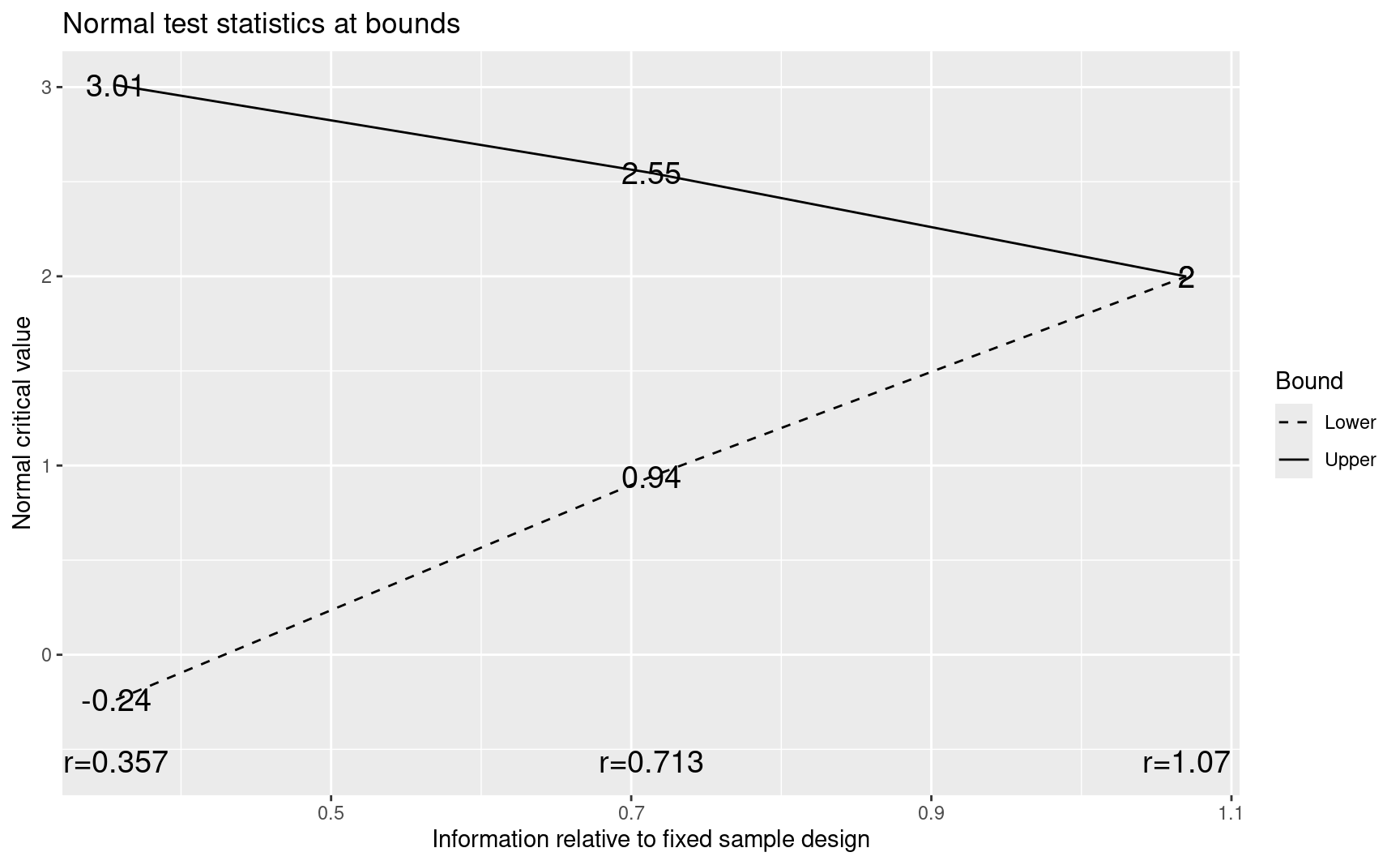
There are several other plots available as will be discussed below. A brief textual summary of the design is obtained with:
summary(x)#> Asymmetric two-sided group sequential design with
#> non-binding futility bound, 3 analyses, sample size 2, 90
#> percent power, 2.5 percent (1-sided) Type I error. Efficacy
#> bounds derived using a Hwang-Shih-DeCani spending function
#> with gamma = -4. Futility bounds derived using a
#> Hwang-Shih-DeCani spending function with gamma = -2.A tabular summary of bounds is generated with
gsBoundSummary(x)
#>                Analysis               Value Efficacy Futility
#>               IA 1: 33%                   Z   3.0107  -0.2387
#>  N/Fixed design N: 0.36         p (1-sided)   0.0013   0.5943
#>                             ~delta at bound   1.5553  -0.1233
#>                         P(Cross) if delta=0   0.0013   0.4057
#>                         P(Cross) if delta=1   0.1412   0.0148
#>               IA 2: 67%                   Z   2.5465   0.9411
#>  N/Fixed design N: 0.71         p (1-sided)   0.0054   0.1733
#>                             ~delta at bound   0.9302   0.3438
#>                         P(Cross) if delta=0   0.0062   0.8347
#>                         P(Cross) if delta=1   0.5815   0.0437
#>                   Final                   Z   1.9992   1.9992
#>  N/Fixed design N: 1.07         p (1-sided)   0.0228   0.0228
#>                             ~delta at bound   0.5963   0.5963
#>                         P(Cross) if delta=0   0.0233   0.9767
#>                         P(Cross) if delta=1   0.9000   0.1000
Above we have seen standard output for gsDesign(). To access individual items of information about what is returned from the above, use names(x) to list the elements of x. Type help(gsDesign) to get full documentation of the class gsDesign returned by the gsDesign() function; the documentation website at https://keaven.github.io/gsDesign/ can also be useful. To view an individual element of x type, for example, x$delta, the standardized effect size for the design (\(\theta\) from ).
Other elements of x can be accessed in the same way, and we will use these to display aspects of designs in further examples. Of particular interest are the elements upper and lower. These are both objects containing multiple variables concerning the upper and lower boundaries and boundary crossing probabilities. Type names(x$upper) to show what these variables are. The upper boundary can be shown with the command x$upper$bound. As an example plot, enter plot(x, plottype=2)) for a power plot. The argument plottype can run from 1 (the default) to 8. The options not already noted plot approximate effect sizes at boundaries (plottype=3; see plottype=8 for hazard ratio), conditional power at boundaries (plottype=4), \(\alpha\)- and \(\beta\)-spending functions (plottype=5), expected sample size by underlying treatment difference (plottype=6), B-values at boundaries (plottype=7), and approximate hazard ratio at boundaries for designs for time-to-event outcomes (plottype=8).
4.4 Applying the default design to the CAPTURE example
The sample size ratios for each analysis relative to a fixed design sample size from Equation 4.1 can be obtained as follows:
x$n.I
#> [1] 0.3566277 0.7132555 1.0698832
These will be applied to each of our examples. Recall from the CAPTURE trial that we had a binomial outcome and wished to detect a reduction in the primary endpoint from a 15% event rate in the control group to a 10% rate in the experimental group. While we consider 80% power elsewhere, we stick with the default of 90% here. A group sequential design with 90% power and 2.5% Type I error has the same bounds as shown previously. The sample size at each analysis is obtained as follows (continuing the code just above):
n.fix <- nBinomial(p1 = 0.15, p2 = 0.1)
n.fix
#> [1] 1834.641
n.fix * x$n.I
#> [1] 654.284 1308.568 1962.852Rounding up to an even number for the final analysis, we see from the above that a while a fixed design requires 1836 patients, employing the default group sequential design inflates the sample size requirement to 1964. Interim analyses would be performed after approximately 655 and 1309 patients.
The group sequential design can be derived directly by replacing the input parameter n.fix with the sample size from a fixed design trial as follows:
The toInteger() function converts the continuous sample size created by gsDesign() to an integer-based sample size design. The argument ratio = 1 in the toInteger() call indicates 1:1 randomization (experimental:control) and will round up the final sample size to an even integer. We will also see below that this yields slightly above the targeted 90% power. Printing the design now replaces the sample size ratio with the actual sample sizes at each analysis.
x
#> Asymmetric two-sided group sequential design with
#> 90 % power and 2.5 % Type I Error.
#> Upper bound spending computations assume
#> trial continues if lower bound is crossed.
#>
#>                   ----Lower bounds----  ----Upper bounds-----
#>   Analysis   N    Z   Nominal p Spend+  Z   Nominal p Spend++
#>          1  654 -0.24    0.4053 0.0148 3.01    0.0013  0.0013
#>          2 1309  0.94    0.8267 0.0289 2.55    0.0054  0.0049
#>          3 1964  2.00    0.9772 0.0563 2.00    0.0228  0.0188
#>      Total                      0.1000                 0.0250
#> + lower bound beta spending (under H1):
#>  Hwang-Shih-DeCani spending function with gamma = -2.
#> ++ alpha spending:
#>  Hwang-Shih-DeCani spending function with gamma = -4.
#>
#> Boundary crossing probabilities and expected sample size
#> assume any cross stops the trial
#>
#> Upper boundary (power or Type I Error)
#>           Analysis
#>    Theta      1      2      3  Total   E{N}
#>   0.0000 0.0013 0.0049 0.0171 0.0233 1146.9
#>   0.0757 0.1410 0.4406 0.3186 0.9001 1452.4
#>
#> Lower boundary (futility or Type II Error)
#>           Analysis
#>    Theta      1      2      3  Total
#>   0.0000 0.4053 0.4294 0.1420 0.9767
#>   0.0757 0.0148 0.0289 0.0562 0.0999
Rather than printing the design as above, we recommend using the summary() function for a textual summary and gsBoundSummary() for a table summarizing bounds.
summary(x)#> Asymmetric two-sided group sequential design with
#> non-binding futility bound, 3 analyses, sample size 1964,
#> 90 percent power, 2.5 percent (1-sided) Type I error.
#> Efficacy bounds derived using a Hwang-Shih-DeCani spending
#> function with gamma = -4. Futility bounds derived using a
#> Hwang-Shih-DeCani spending function with gamma = -2.x |> gsBoundSummary(deltaname = "Risk difference")
#> Analysis Value Efficacy Futility
#> IA 1: 33% Z 3.0113 -0.2397
#> N: 654 p (1-sided) 0.0013 0.5947
#> ~Risk difference at bound 0.0778 -0.0062
#> P(Cross) if Risk difference=0 0.0013 0.4053
#> P(Cross) if Risk difference=0.05 0.1410 0.0148
#> IA 2: 67% Z 2.5468 0.9413
#> N: 1309 p (1-sided) 0.0054 0.1733
#> ~Risk difference at bound 0.0465 0.0172
#> P(Cross) if Risk difference=0 0.0062 0.8347
#> P(Cross) if Risk difference=0.05 0.5815 0.0437
#> Final Z 1.9992 1.9992
#> N: 1964 p (1-sided) 0.0228 0.0228
#> ~Risk difference at bound 0.0298 0.0298
#> P(Cross) if Risk difference=0 0.0233 0.9767
#> P(Cross) if Risk difference=0.05 0.9001 0.0999The risk difference at bound line gives an approximate minimum difference in event rates that will result in crossing a bound. This should work well when the average risk across arms is the same as the design average, in this case (0.15 + 0.1) / 2 = 0.125. For instance, looking at an observed risk difference of approximately 0.0078 at interim 1 when the average risk of the 2 arms is approximately 0.125 yields a Z-statistic close to that in the above table (3.01)
# Risk reduction uses x1, n1 for control,
# x2, n2 for experimental group.
testBinomial(
  x1 = round((0.125 + 0.0778 / 2) * 327), # 54 events
  x2 = round((0.125 - 0.0778 / 2) * 327), # 28 events
  n1 = 327, n2 = 327
)
#> [1] 3.070134
However, if the overall absolute risk is different this approximation will not work well:
# Lower risk
testBinomial(
  x1 = round((0.1 + 0.0778 / 2) * 327), # 45 events
  x2 = round((0.1 - 0.0778 / 2) * 327), # 20 events
  n1 = 327, n2 = 327
)
#> [1] 3.267492
# Higher risk
testBinomial(
x1 = round((0.15 + 0.0778 / 2) * 327), # 62 events
x2 = round((0.15 - 0.0778 / 2) * 327), # 36 events
n1 = 327, n2 = 327
)
#> [1] 2.8484714.4.1 Simulation of a binomial design
Testing at each analysis can be performed using the Miettinen and Nurminen (Miettinen and Nurminen 1985) method. Simulation to verify the normal approximation is adequate for comparing binomial event rates can be performed using the functions simBinomial and testBinomial using the CAPTURE fixed design from above with N = 1836. This is only set up for fixed design, but suggests that the normal approximations used for power and Type I error calculations are quite good.
# Show that power is 90% using simulation
Z <- simBinomial(
  nsim = 100000,
  p1 = 0.15,
  p2 = 0.1,
  n1 = 1836 / 2,
  n2 = 1836 / 2
)
mean(Z >= qnorm(0.975))
#> [1] 0.90151
Under the null hypothesis, we have:
# Show that Type I error is 2.5%
Z <- simBinomial(
  nsim = 100000,
  p1 = 0.125,
  p2 = 0.125,
  n1 = 1836 / 2,
  n2 = 1836 / 2
)
mean(Z >= qnorm(0.975))
#> [1] 0.02444
4.4.2 Applying the default design to the noninferiority example
The fixed noninferiority design for a binomial comparison is the same as above, only changing the nBinomial() call to
n.fix <- nBinomial(p1 = 0.677, p2 = 0.677, delta0 = -0.07)# delta0 is minus the non-inferiority margin,
# in this case, we are trying to rule out
# a risk increase over control of 0.07 or more.
ni_design <- gsDesign(
n.fix = n.fix,
delta0 = -0.07,
delta1 = 0,
endpoint = "binomial"
) |> toInteger(ratio = 1)
ni_design |> gsBoundSummary(deltaname = "Risk difference")
#> Analysis Value Efficacy Futility
#> IA 1: 33% Z 3.0107 -0.2386
#> N: 668 p (1-sided) 0.0013 0.5943
#> ~Risk difference at bound 0.0389 -0.0786
#> P(Cross) if Risk difference=-0.07 0.0013 0.4057
#> P(Cross) if Risk difference=0 0.1412 0.0148
#> IA 2: 67% Z 2.5465 0.9412
#> N: 1336 p (1-sided) 0.0054 0.1733
#> ~Risk difference at bound -0.0049 -0.0459
#> P(Cross) if Risk difference=-0.07 0.0062 0.8347
#> P(Cross) if Risk difference=0 0.5815 0.0437
#> Final Z 1.9992 1.9992
#> N: 2004 p (1-sided) 0.0228 0.0228
#> ~Risk difference at bound -0.0283 -0.0283
#> P(Cross) if Risk difference=-0.07 0.0233 0.9767
#> P(Cross) if Risk difference=0 0.9000 0.1000We examine the risk difference approximations at the efficacy and futility bounds at analysis 2. First, for the futility bound 468 events in the experimental group vs. 437 in the control is a big enough increase in risk to declare futility for an eventual non-inferiority finding with an allowable increase in risk of no more than 0.07:
testBinomial(
  delta0 = -0.07, n1 = 668, n2 = 668,
  x1 = round((0.677 - 0.0459 / 2) * 668), # 437 events
  x2 = round((0.677 + 0.0459 / 2) * 668) # 468 events
)
#> [1] 0.9244426
For the efficacy bound 454 experimental events in the experimental group vs. 451 in the control group is sufficient at the second interim to declare non-inferiority (i.e., rule out more than a 0.07 risk difference in the experimental group vs. control):
testBinomial(
  delta0 = -0.07, n1 = 668, n2 = 668,
  x1 = round((0.677 - 0.0049 / 2) * 668), # 451 events
  x2 = round((0.677 + 0.0049 / 2) * 668) # 454 events
)
#> [1] 2.564413
We see these approximations are quite reasonable when to overall average event rate is 0.677.
4.5 Applying the default design to the cancer trial example
For trials with time-to-event outcomes, the variable n.fix in gsDesign() needed is the number of events from a fixed design trial. The reader may wish to refer to Jennison and Turnbull (Jennison and Turnbull 2000) for further background; we also discuss distributional assumptions further in Section 7.3.2. We begin with the code from the fixed design trial for the cancer trial example from Section 1.6. Next, we call to gsDesign() with n.fix equal to the number of events for a fixed trial design. The value ssratio, the sample size ratio at each analysis compared to the fixed design sample size is then shown. Note that the values are the same as shown in the first output of this example above. The inflation in the total sample size is the same as for the number of events required if enrollment duration and dropout rates are not changed; that is, the sample size required for a group sequential design with the default interim analysis plan is inflated by multiplying by 1.07. In the last line of code below, we demonstrate a plot showing the approximate hazard ratios required to cross a bound.
The overall design summary is:
summary(y)#> Asymmetric two-sided group sequential design with
#> non-binding futility bound, 3 analyses, sample size 353, 90
#> percent power, 2.5 percent (1-sided) Type I error. Efficacy
#> bounds derived using a Hwang-Shih-DeCani spending function
#> with gamma = -4. Futility bounds derived using a
#> Hwang-Shih-DeCani spending function with gamma = -2.The boundary summary table is obtained with:
y |> gsBoundSummary(deltaname = "HR")
#>   Analysis            Value Efficacy Futility
#>  IA 1: 33%                Z   3.0107  -0.2387
#>     N: 118      p (1-sided)   0.0013   0.5943
#>                ~HR at bound   0.5736   1.0451
#>            P(Cross) if HR=0   0.0013   0.4057
#>            P(Cross) if HR=1   0.1412   0.0148
#>  IA 2: 67%                Z   2.5465   0.9411
#>     N: 235      p (1-sided)   0.0054   0.1733
#>                ~HR at bound   0.7172   0.8844
#>            P(Cross) if HR=0   0.0062   0.8347
#>            P(Cross) if HR=1   0.5815   0.0437
#>      Final                Z   1.9992   1.9992
#>     N: 353      p (1-sided)   0.0228   0.0228
#>                ~HR at bound   0.8081   0.8081
#>            P(Cross) if HR=0   0.0233   0.9767
#>            P(Cross) if HR=1   0.9000   0.1000
In order to update the design, we consider the planned maximum number of events and the achieved events at each analysis. For example, if we have 125, 250 and 365 events at the 3 analyses we update bounds as below. Note that if this is a mixture of planned (later analyses) and actual events (earlier analyses), this is fine. Is also possible to have fewer or more analyses than in the original design.
# Update time-to-event group sequential design
yu <- gsDesign(
  # Number of analyses
  k = 3,
  # Type I error
  alpha = y$alpha,
  # Type II error (1 - power)
  beta = y$beta,
  # Final planned event count
  maxn.IPlan = max(y$n.I),
  # Actual event counts at analyses
  n.I = c(125, 250, 364),
  # Bound type (in this case, non-binding futility)
  test.type = y$test.type,
  # Efficacy spending function
  sfu = y$upper$sf,
  # Parameter(s) for beta-spending (futility)
  sfupar = y$upper$param,
  # Futility spending function
  sfl = y$lower$sf,
  # Futility spending function parameter(s)
  sflpar = y$lower$param,
  # Standardized effect size
  delta = y$delta,
  # Natural parameter under H1 (ln(HR))
  delta1 = y$delta1,
  # Natural parameter under H0 (ln(1) = 0 for superiority)
  delta0 = y$delta0
)
gsBoundSummary(
  yu,
  deltaname = "HR",
  logdelta = TRUE,
  Nname = "Events",
  digits = 4,
  exclude = c(
    "Z", "B-value", "CP", "CP H1", "PP", "~HR at bound",
    # Following line deletes probability of boundary crossing
    # under null and alternate hypothesis; this must be customized,
    # if needed
    paste0("P(Cross) if HR=", c("0.7", "1"))
  )
)
#>     Analysis               Value Efficacy Futility
#>    IA 1: 36%         p (1-sided)   0.0015   0.5565
#>  Events: 125            Spending   0.0015   0.0162
#>              P(Cross) if HR=2.72   0.1641   0.0162
#>    IA 2: 71%         p (1-sided)   0.0066   0.1381
#>  Events: 250            Spending   0.0061   0.0329
#>              P(Cross) if HR=2.72   0.6414   0.0491
#>        Final         p (1-sided)   0.0223   0.0223
#>  Events: 364            Spending   0.0175   0.0509
#>              P(Cross) if HR=2.72   0.9046   0.0954
To avoid confusion we have limited the number of parameters displayed as only the 1-sided nominal \(p\)-value (p (1-sided)) should be needed to evaluate boundary crossing. Different parameters can be excluded from the table by changing the list passed to the exclude argument.
4.6 Further properties of designs
We consider further the design for a time-to-event variable assuming proportional hazards. To understand properties of the design better, we consider selected summary plots and we also demonstrate the gsProbability() function. First, we plot the operating characteristics for a larger set of hazard ratios than in the standard printout above.
plot(y, plottype = "Power")
#> Warning: Using `size` aesthetic for lines was deprecated in ggplot2
#> 3.4.0.
#> ℹ Please use `linewidth` instead.
#> ℹ The deprecated feature was likely used in the gsDesign
#>   package.
#>   Please report the issue at
#>   <https://github.com/keaven/gsDesign/issues>.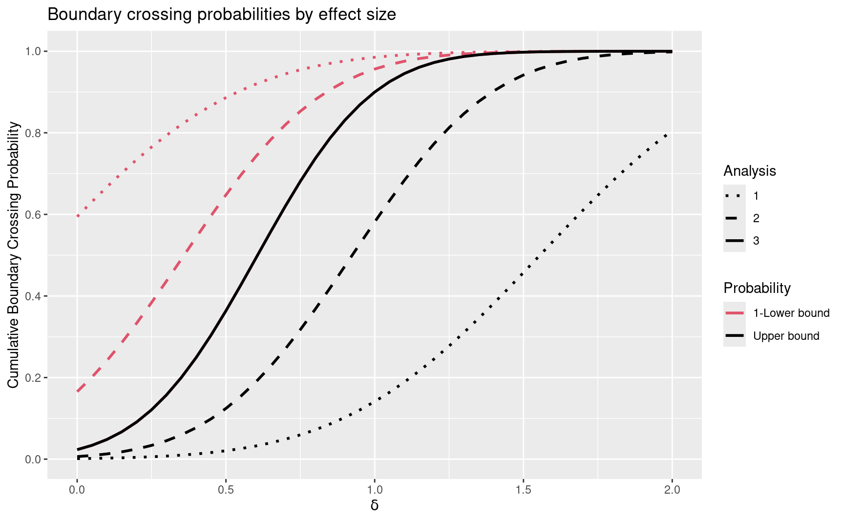
The solid black line is of most interest as it shows the power of the design for different underlying hazard ratios. The dotted black line shows the probability of crossing the efficacy bound at the first interim, while the dashed black line shows the cumulative probability of crossing at the first or second interim. The red dotted line shows 1 minus the probability of crossing the futility bound at the first interim analysis for different hazard ratios. The red dashed line show 1 minus the cumulative probability of crossing the futility bound at the first or second interim analysis. For each hazard ratio, the lines divide the outcomes vertically into mutually exclusive possibilities for the trial; in this case (from bottom to top) 1) probability of first cross being efficacy at interim 1 (below dotted black line), 2) first cross being efficacy at interim 2 (between dotted and dashed black lines), 3) first crossing being efficacy at final analysis (between dashed and solid black lines), 4) first crossing being futility at final analysis (between solid black and dashed red lines), 5) first crossing being futility at analysis 2 (between dashed and dotted red lines), and 6) first crossing being futility at analysis 1 (above red dotted red line).
Note that the plot() function for the gsDesign class (used here) is an extension of the standard plot() function, and thus allows use of many of its parameters, such as line width (lwd), line type (lty), plot titles and axis labels.
The first two lines of code below demonstrate that a group sequential design generated by gsDesign() or gsSurv() can be input to gsProbability() to obtain boundary crossing probabilities for an extended set of parameter values. The theta values in the output make more sense in this case when they are computed relative to the effect size (log hazard ratio) y$delta1= 1 or hazard ratio exp(y$delta1)= 2.72for which the trial is powered; this is more easily seen in the power plot above than in the printout below.
hr <- seq(0.4, 1.1, 0.1)
yp <- gsProbability(theta = log(hr) * y$delta / y$delta1, d = y)
yp
#> Asymmetric two-sided group sequential design with
#> 90 % power and 2.5 % Type I Error.
#> Upper bound spending computations assume
#> trial continues if lower bound is crossed.
#>
#>                  ----Lower bounds----  ----Upper bounds-----
#>   Analysis  N    Z   Nominal p Spend+  Z   Nominal p Spend++
#>          1 118 -0.24    0.4057 0.0148 3.01    0.0013  0.0013
#>          2 235  0.94    0.8267 0.0289 2.55    0.0054  0.0049
#>          3 353  2.00    0.9772 0.0563 2.00    0.0228  0.0188
#>      Total                     0.1000                 0.0250
#> + lower bound beta spending (under H1):
#>  Hwang-Shih-DeCani spending function with gamma = -2.
#> ++ alpha spending:
#>  Hwang-Shih-DeCani spending function with gamma = -4.
#>
#> Boundary crossing probabilities and expected sample size
#> assume any cross stops the trial
#>
#> Upper boundary (power or Type I Error)
#>           Analysis
#>     Theta      1      2      3  Total  E{N}
#>   -0.1637 0.0000 0.0000 0.0000 0.0000 124.7
#>   -0.1239 0.0000 0.0000 0.0000 0.0000 133.5
#>   -0.0913 0.0000 0.0000 0.0001 0.0001 145.0
#>   -0.0637 0.0001 0.0002 0.0005 0.0008 158.6
#>   -0.0399 0.0003 0.0007 0.0023 0.0033 173.6
#>   -0.0188 0.0007 0.0021 0.0071 0.0098 189.5
#>    0.0000 0.0013 0.0049 0.0171 0.0233 205.6
#>    0.0170 0.0024 0.0101 0.0343 0.0467 221.4
#>
#> Lower boundary (futility or Type II Error)
#>           Analysis
#>     Theta      1      2      3  Total
#>   -0.1637 0.9376 0.0621 0.0003 1.0000
#>   -0.1239 0.8650 0.1329 0.0021 1.0000
#>   -0.0913 0.7734 0.2175 0.0089 0.9999
#>   -0.0637 0.6743 0.2997 0.0252 0.9992
#>   -0.0399 0.5766 0.3662 0.0538 0.9967
#>   -0.0188 0.4861 0.4098 0.0942 0.9902
#>    0.0000 0.4057 0.4290 0.1420 0.9767
#>    0.0170 0.3361 0.4264 0.1909 0.9533
Say we wish to compare values for y$theta = 0.2559 to the plot above; we can translate to the HR scale with
exp(yp$theta[3] * y$delta1 / y$delta)
#> [1] 0.6
The we see the incremental probabilities described for the plot when HR = 0.6 are (from the table above): 0.4029, 0.5141, 0.0787, 0.0018, 0.0012, and 0.0013, respectively. Thus, the most likely outcomes are positive efficacy findings at interim 1 or 2 when the true underlying HR=0.6.
p <- plot(y, plottype = 6)
p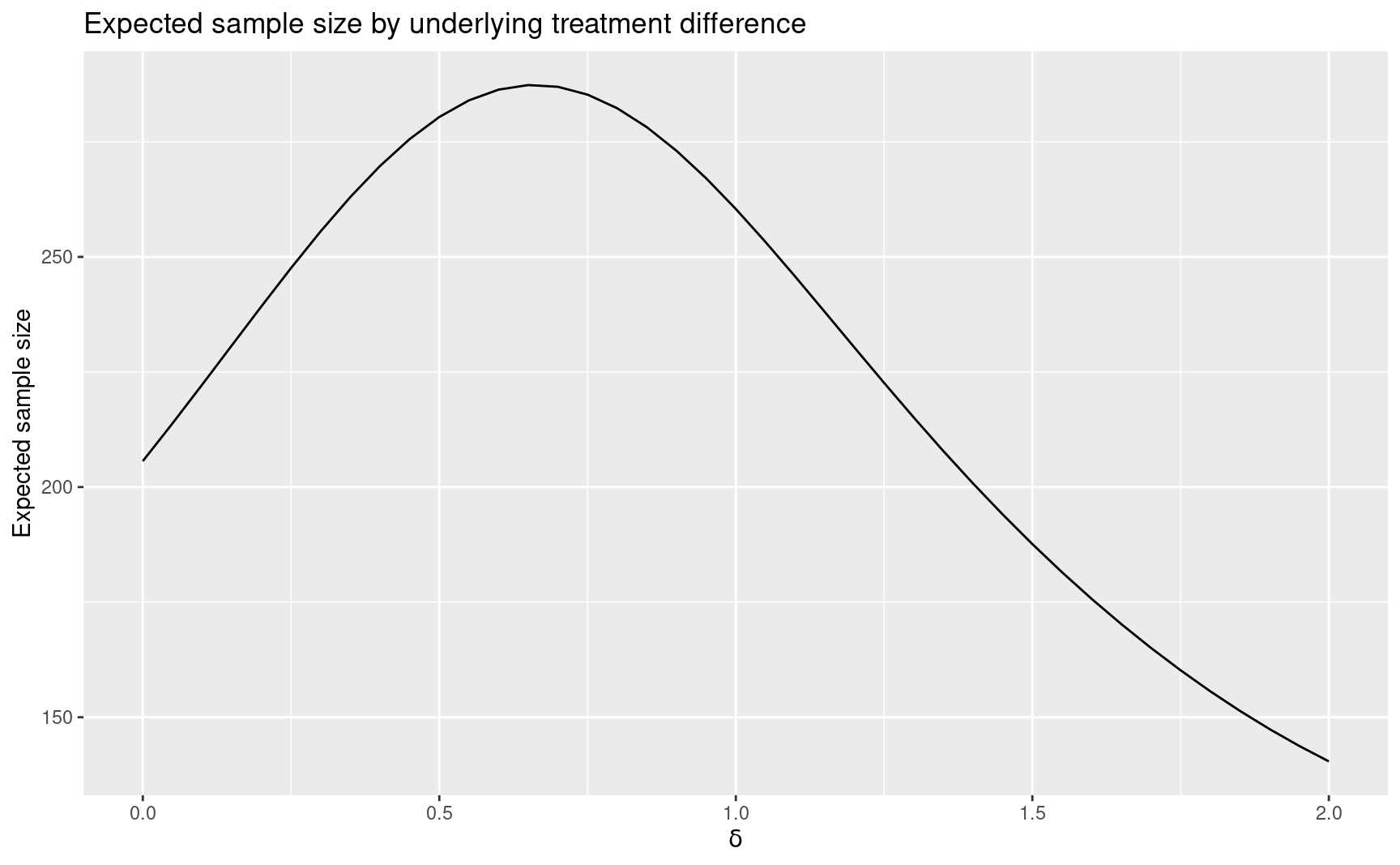
Following is a plot with the approximate hazard ratio required to cross each bound. The \(y\)-axis shows the expected number of events in the analysis where a bound is first crossed or, if no bound is crossed, the final analysis. relative to a fixed design trial when the sample size ratio is computed; if we had input a fixed design sample size, the \(y\)-axis would show the actual expected sample size. This plot demonstrates the ability of a group sequential design to appropriate adapt sample size to come to an appropriate conclusion depending on the true treatment effect.
p <- plot(y, plottype = "HR")
p