8  Spending functions

8.1 Spending function definitions

For any given \(0 < \alpha < 1\), we define a non-decreasing function \(f(t; \alpha)\) for \(t \geq 0\) with \(\alpha(0) = 0\) and for \(t \geq 1\), \(f(t; \alpha) = \alpha\). For \(i = 1, 2, \ldots, K\), we define \(t_i=I_{i}/I_{K}\) and then set \(\alpha_i(0)\) through the equation

\[ f(t_i; \alpha) = \sum_{j=1}^{i}\alpha_{j}(0). \]

We consider a spending function proposed by Lan and DeMets (Lan and DeMets 1983) to approximate a Pocock bound.

\[ f(t; \alpha)=\alpha\log(1+(e-1)t) \]

This spending function is implemented in the function sfLDPocock. We again consider a 2-sided design with equally spaced analyses, \(t_i = i/4\), \(i = 1, 2, 3, 4\). The values for \(\alpha_i(0)\) are obtained as follows:

library(gsDesign)

sfLDPocock(alpha = 0.025, t = 1:4 / 4)$spend
#> [1] 0.00893435 0.01550286 0.02069972 0.02500000

We will discuss the exact nature of this call to sfLDPocock in Section 8.5 below. We now derive a design for the CAPTURE study using this spending function

n.fix <- nBinomial(p1 = 0.15, p2 = 0.1, beta = 0.2)
x <- gsDesign(
  k = 4,
  test.type = 2,
  n.fix = n.fix,
  sfu = sfLDPocock,
  beta = 0.2
)
cumsum(x$upper$prob[, 1])
#> [1] 0.00893435 0.01550287 0.02069973 0.02500001

The boundary crossing probabilities under the assumption of no treatment difference are in x$upper$prob[,1] and there cumulative totals are produced by the above call to cumsum(). Note that these values match those produced by the call to sfLDPocock above. Next we compare the bounds produced by this design with the actual Pocock bounds to see they are nearly identical:

xPocock <- gsDesign(
  k = 4,
  test.type = 2,
  n.fix = n.fix,
  sfu = "Pocock",
  beta = 0.2
)
x$upper$bound
#> [1] 2.368328 2.367524 2.358168 2.350030

xPocock$upper$bound
#> [1] 2.361298 2.361298 2.361298 2.361298

The reader may wish to compare the O’Brien-Fleming design presented in Section 6.2 using the spending function sfLDOF, which implements a spending function proposed by Lan and DeMets (Lan and DeMets 1983) to approximate this design:

\[ \alpha_i(t)=2\left(1-\Phi\left(\frac{\Phi^{-1}(\alpha/2)}{\sqrt{t}}\right)\right) \]

You will see that this approximation is not as good as the Pocock bound approximation.

8.2 Spending function families

The function \(f(t;\alpha)\) may be generalized to a family \(f(t;\alpha,\gamma)\) of spending functions using one or more parameters. For instance, the default Hwang-Shih-DeCani spending function family is defined for \(0\leq t\leq 1\) and any real \(\gamma\) by

\[ f(t;\alpha, \gamma)= % \begin{array} [c]{cc}% \alpha\frac{1-\exp(-\gamma t)}{1-\exp(-\gamma)}, & \gamma\neq 0\\ \alpha t, & \gamma=0 \end{array} \]

The boundary crossing probabilities \(\alpha_i^{+}(\theta)\) and \(\beta_i(\theta)\) may be defined in a similar fashion, \(i=1,2,\ldots,K\) with the same or different spending functions \(f\) where:

\[\begin{align} f(t_i;\alpha) & = &\sum_{j=1}^{i}\alpha_{j}^{+}(0)\\ f(t_i;\beta(\theta)) & = & \sum_{j=1}^{i}\beta_j(\theta) \end{align}\]

The argument test.type in gsDesign() provides two options for how to use \(f(t_i;\beta(\theta))\) to set lower bounds. For test.type=2, 5 and 6, lower boundary values are set under the null hypothesis by specifying \(\beta(t;0),\) \(0\leq t\). For test.type=3 and 4, we compute lower boundary values under the alternative hypothesis by specifying \(\beta(t;\delta)\), \(0\leq t\). \(\beta(t;\delta)\) is referred to as the \(\beta\)-spending function and the value \(\beta_{i}(\delta)\) is referred to as the amount of \(\beta\) (Type II error rate) spent at analysis \(i\), \(1\leq i\leq K\).

Standard published spending functions commonly used for group sequential design are included as part of the gsDesign package. Several ‘new’ spending functions are included that are of potential interest. Users can also write their own spending functions to pass directly to gsDesign(). Available spending functions and the syntax for writing a new spending function are documented here. We begin here with simple examples of how to apply standard spending functions in calls to gsDesign(). This may be as far as many readers may want to read. However, for those interested in more esoteric spending functions, full documentation of the extensive spending function capabilities available is included. Examples for each type of spending function in the package are included in the online help documentation.

8.3 Spending function basics

The parameters sfu and sfl are used to set spending functions for the upper and lower bounds, respectively, each having a default value of sfHSD, the Hwang-Shih-DeCani spending function. The default parameter for the upper bound is \(\gamma = -4\) to produce a conservative, O’Brien-Fleming-like bound. The default for the lower bound is \(\gamma = -2\), a less conservative bound. This design was presented at some length in Section 4.1.

To change these to \(-3\) (less conservative than an O’Brien-Fleming bound) and \(1\) (an aggressive Pocock-like bound), respectively, requires the parameter sfupar for the upper bound and sflpar for the lower bound: Next we consider some simple alternatives to the default spending function parameters. The Kim-DeMets function, sfPower(), with upper bound parameter \(\rho = 3\) (a conservative, O’Brien-Fleming-like bound) and lower bound parameter \(\rho = 0.75\) (an aggressive, Pocock-like bound) requires resetting the upper bound spending function sfu and the lower bound spending function sfl. In the first code line following, we replace lower and upper spending function parameters with \(1\) and \(-2\), respectively; the default Hwang-Shih-DeCani spending function family is still used. In the second line, we specify a Kim-DeMets (power) spending function for both the lower bound (with the parameters sfl=sfPower and sflpar=2) and the upper bounds (with the parameters sfu=sfPower and sfupar=3). Then we compare bounds from the three designs. Bounds for the power spending function design are quite comparable to the default design. Generally, choosing between these two spending function families is somewhat arbitrary. The alternate Hwang-Shih-DeCani design uses more aggressive stopping boundaries. The last lines below show that sample size inflation from a fixed design is about 25% for the the design with more aggressive stopping boundaries compared to about 7% for each of the other designs.

x <- gsDesign()
xHSDalt <- gsDesign(
  sflpar = 1,
  sfupar = -2
)
xKD <- gsDesign(
  sfl = sfPower,
  sflpar = 2,
  sfu = sfPower,
  sfupar = 3
)
x$upper$bound
#> [1] 3.010739 2.546531 1.999226

xHSDalt$upper$bound
#> [1] 2.677524 2.385418 2.063740

xKD$upper$bound
#> [1] 3.113017 2.461933 2.008705

x$lower$bound
#> [1] -0.2387240  0.9410673  1.9992264

xHSDalt$lower$bound
#> [1] 0.3989131 1.3302942 2.0637399

xKD$lower$bound
#> [1] -0.3497490  0.9822542  2.0087052

x$n.I[3]
#> [1] 1.069883

xHSDalt$n.I[3]
#> [1] 1.254268

xKD$n.I[3]
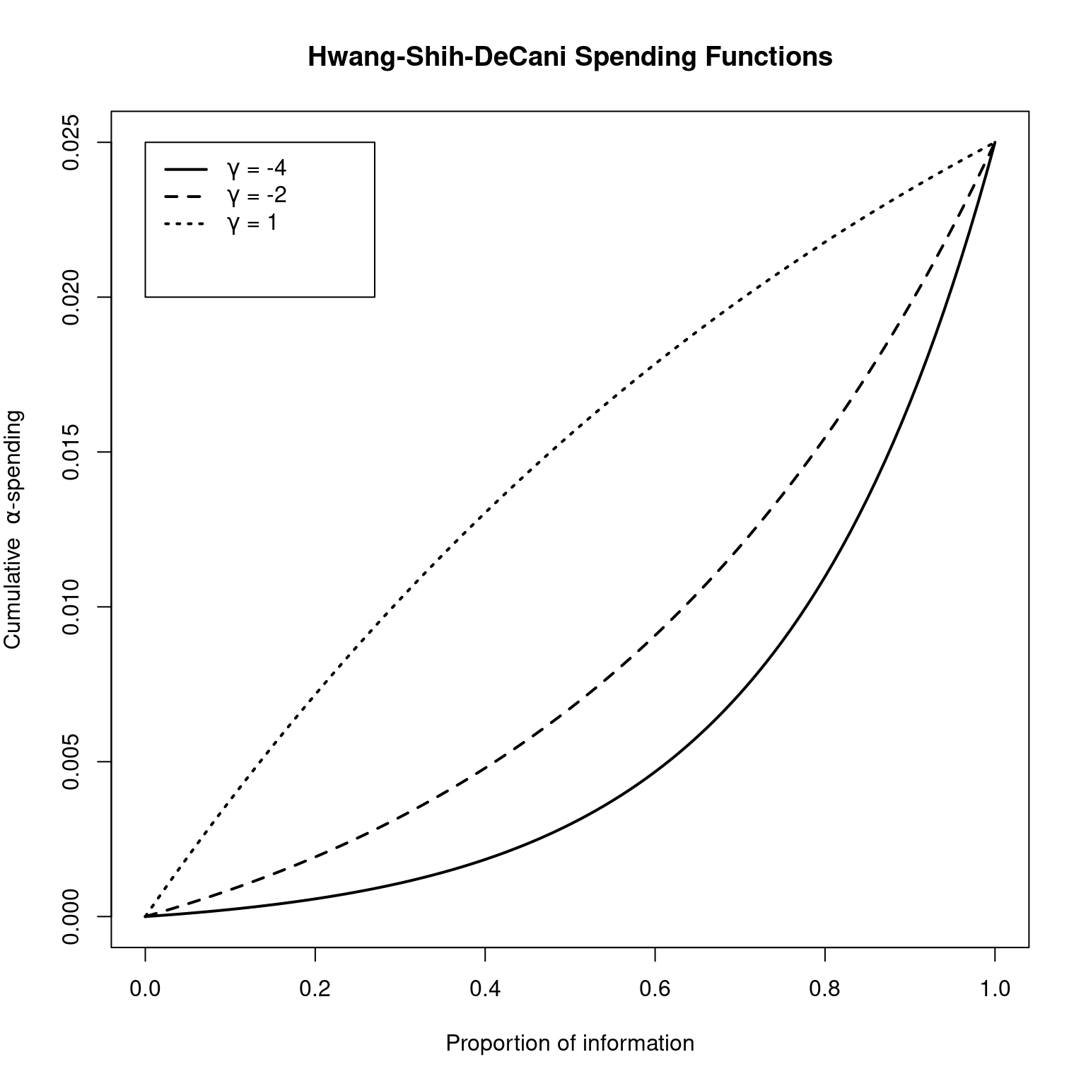
#> [1] 1.071011

Following is example code to plot Hwang-Shih-DeCani spending functions for three values of the \(\gamma\) parameter. The first two \(\gamma\) values are the defaults for upper bound spending (\(\gamma = -4\); a conservative bound somewhat similar to an O’Brien-Fleming bound) and lower bound spending (\(\gamma = -2\); a less conservative bound). The third (\(\gamma = 1\)) is included as it approximates a Pocock stopping rule; see Hwang, Shih and DeCani (Hwang, Shih, and De Cani 1990). The Hwang-Shih-DeCani spending function class implemented in the function sfHSD() may be sufficient for designing many clinical trials without considering the other spending function forms available in this package. The three parameters in the calls to sfHSD() below are the total Type I error, values for which the spending function is evaluated (and later plotted), and the \(\gamma\) parameter for the Hwang-Shih-DeCani design. The code below yields the plot in Figure 8.1 (note the typesetting of Greek characters!).

plot(0:100 / 100, sfHSD(0.025, 0:100 / 100, -4)$spend,
  type = "l", lwd = 2,
  xlab = "Proportion of information",
  ylab = expression(paste("Cumulative \ ", alpha, "-spending")),
  main = "Hwang-Shih-DeCani Spending Functions"
)
lines(
  0:100 / 100,
  sfHSD(0.025, 0:100 / 100, -2)$spend,
  lty = 2,
  lwd = 2
)
lines(
  0:100 / 100,
  sfHSD(0.025, 0:100 / 100, 1)$spend,
  lty = 3,
  lwd = 2
)
legend(
  x = c(0.0, 0.27), y = 0.025 * c(0.8, 1), lty = 1:3, lwd = 2,
  legend = c(
    expression(paste(gamma, " = -4")),
    expression(paste(gamma, " = -2")),
    expression(paste(gamma, " = 1"))
  )
)

Figure 8.1

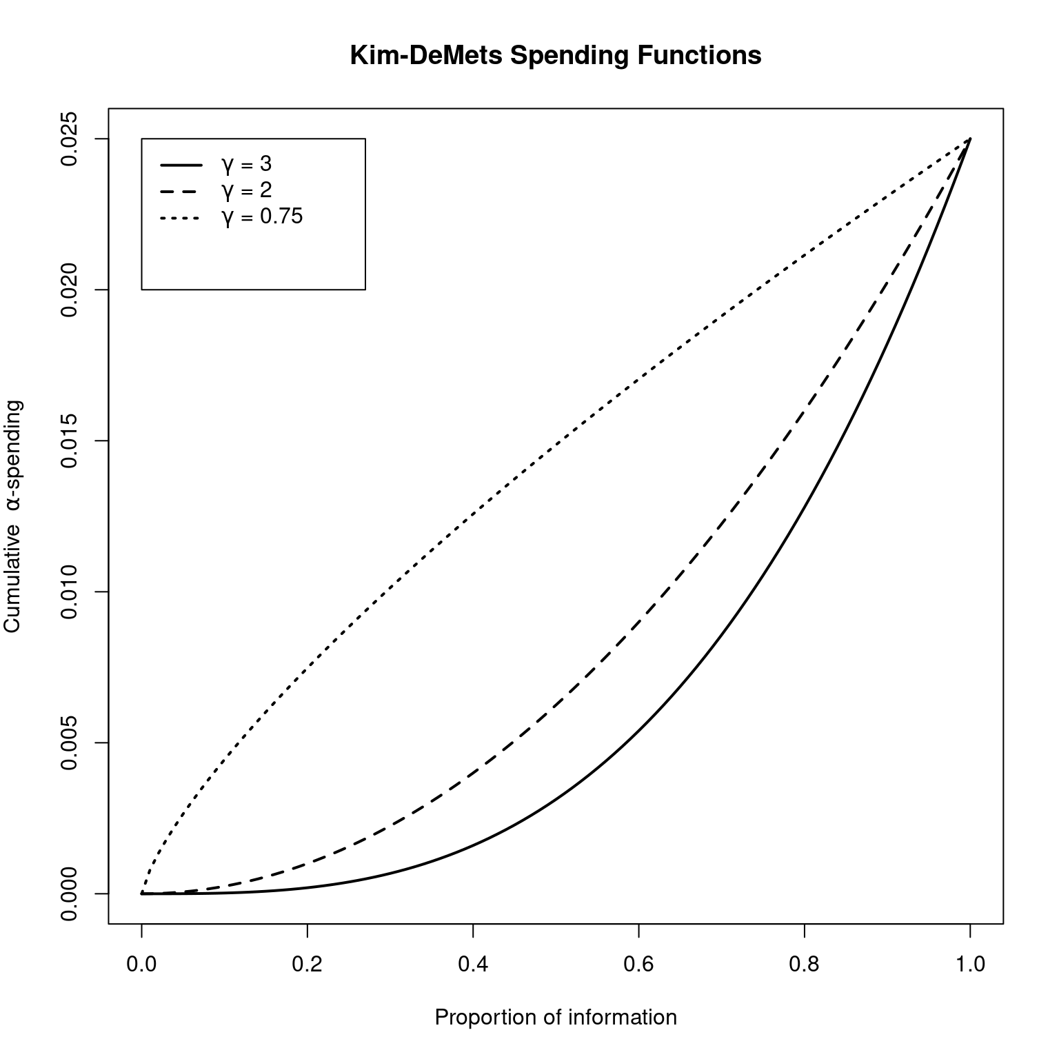
Similarly, Jennison and Turnbull (Jennison and Turnbull 2000), suggest that the Kim-DeMets spending function is flexible enough to suit most purposes. To compare the Kim-DeMets family with the Hwang-Shih-DeCani family just demonstrated, substitute sfPower() instead of sfHSD(); use parameter values \(3\), \(2\) and \(0.75\) to replace the values \(-4\),\(-2\), and \(1\) in the code shown above:

plot(0:100 / 100, sfPower(0.025, 0:100 / 100, 3)$spend,
  type = "l", lwd = 2,
  xlab = "Proportion of information",
  ylab = expression(paste("Cumulative \ ", alpha, "-spending")),
  main = "Kim-DeMets Spending Functions"
)
lines(
  0:100 / 100,
  sfPower(0.025, 0:100 / 100, 2)$spend,
  lty = 2,
  lwd = 2
)
lines(
  0:100 / 100,
  sfPower(0.025, 0:100 / 100, 0.75)$spend,
  lty = 3,
  lwd = 2
)
legend(
  x = c(0.0, 0.27), y = 0.025 * c(0.8, 1), lty = 1:3, lwd = 2,
  legend = c(
    expression(paste(gamma, " = 3")),
    expression(paste(gamma, " = 2")),
    expression(paste(gamma, " = 0.75"))
  )
)

Figure 8.2

8.4 Resetting timing of analyses

When designed with a spending function, the timing and number of analyses may be altered during the course of the trial. This is very easily handled in the gsDesign() routine using the input arguments n.I and maxn.IPlan. We demonstrate this by example. Suppose a trial was originally designed with the call:

x <- gsDesign(k = 5, n.fix = 800)
x$upper$bound
#> [1] 3.252668 2.986046 2.691657 2.373666 2.025321

x$n.I
#> [1] 176.21 352.42 528.63 704.84 881.05

The second and third lines above show the planned upper bounds and sample sizes at analyses. Suppose that when executed the final interim was skipped, the first 2 interims were completed on time, the third interim was completed at 575 patients (instead of 529 as originally planned), the fourth interim was skipped, and the final analysis was performed after 875 patients (instead of after 882 as originally planned). The boundaries for the analyses can be obtained as follows:

gsDesign(
  k = 4,
  n.fix = 800,
  n.I = c(177, 353, 575, 875),
  maxn.IPlan = x$n.I[x$k]
)
#> Asymmetric two-sided group sequential design with
#> 90 % power and 2.5 % Type I Error.
#> Upper bound spending computations assume
#> trial continues if lower bound is crossed.
#> 
#>                  ----Lower bounds----  ----Upper bounds-----
#>   Analysis  N    Z   Nominal p Spend+  Z   Nominal p Spend++
#>          1 177 -0.90    0.1851 0.0077 3.25    0.0006  0.0006
#>          2 353 -0.03    0.4863 0.0115 2.99    0.0014  0.0013
#>          3 575  0.90    0.8149 0.0229 2.59    0.0048  0.0040
#>          4 875  2.01    0.9779 0.0563 2.01    0.0221  0.0184
#>      Total                     0.0984                 0.0243 
#> + lower bound beta spending (under H1):
#>  Hwang-Shih-DeCani spending function with gamma = -2.
#> ++ alpha spending:
#>  Hwang-Shih-DeCani spending function with gamma = -4.
#> 
#> Boundary crossing probabilities and expected sample size
#> assume any cross stops the trial
#> 
#> Upper boundary (power or Type I Error)
#>           Analysis
#>    Theta      1      2      3      4  Total  E{N}
#>   0.0000 0.0006 0.0013 0.0040 0.0168 0.0227 480.1
#>   0.1146 0.0422 0.1683 0.3601 0.3323 0.9028 631.5
#> 
#> Lower boundary (futility or Type II Error)
#>           Analysis
#>    Theta      1      2      3      4  Total
#>   0.0000 0.1851 0.3197 0.3219 0.1507 0.9773
#>   0.1146 0.0077 0.0115 0.0229 0.0551 0.0972

This design now has slightly higher power (90.4%) than the originally planned 90%. This is because the final boundary was lowered relative to the original plan when the \(\alpha\)-spending planned for the fourth interim was saved for the final analysis by skipping the final interim. Note that all of the arguments for the original design must be supplied when the study is re-designed—in addition to adding n.I, which may have the same number, fewer, or more interim analyses compared to the original plan. If the sample size for the final analysis is changed, maxn.IPlan should be passed in as the original final sample size in order to appropriately assign \(\alpha\)- and \(\beta\)-spending for the interim analyses.

8.5 Advanced spending function details

8.5.1 Spending functions as arguments

Except for the "OF", "Pocock" and "WT" examples given in Section 6.2, a spending function passed to gsDesign() through the arguments (upper bound) and (lower bound) must have the following calling sequence:

sfname(alpha, t, param)

where sfname is an arbitrary name for a spending function available from the package or written by the user. The arguments are as follows:

• alpha: a real value (\(0 < \mathtt{alpha} < 1\)). The total error spending for the boundary to be determined. This would be replaced with the following values from a call to gsDesign(): alpha for the upper bound, and either beta (for test.type = 3 or 4) or astar (for test.type = 5 or 6) for the lower bound.
• t: a vector of arbitrary length \(m\) of real values, \(0 \leq t_{1} < t_{2} < \ldots t_{m}\leq1\). Specifies the proportion of spending for which values of the spending function are to be computed.
• param: for all cases here, this is either a real value or a vector of real values. One or more parameters that (with the parameter alpha) fully specify the spending function. This is specified in a call to gsDesign() with sfupar for the upper bound and sflpar for the lower bound.

The value returned is of the class spendfn which was described in Chapter 8, The spendfn Class.

The following code and output demonstrate that the default value sfHSD for the upper and lower spending functions sfu and sfl is a function:

sfHSD
#> function (alpha, t, param) 
#> {
#>     checkScalar(alpha, "numeric", c(0, Inf), c(FALSE, FALSE))
#>     checkScalar(param, "numeric", c(-40, 40))
#>     checkVector(t, "numeric", c(0, Inf), c(TRUE, FALSE))
#>     t[t > 1] <- 1
#>     x <- list(name = "Hwang-Shih-DeCani", param = param, parname = "gamma", 
#>         sf = sfHSD, spend = if (param == 0) t * alpha else alpha * 
#>             (1 - exp(-t * param))/(1 - exp(-param)), bound = NULL, 
#>         prob = NULL)
#>     class(x) <- "spendfn"
#>     x
#> }
#> <bytecode: 0x560bb5765428>
#> <environment: namespace:gsDesign>

Table 8.1 summarizes many spending functions available in the package. A basic description of each type of spending function is given. The table begins with standard spending functions followed by two investigational spending functions: sfExponential() and sfLogistic(). These spending functions are discussed further in Section 8.5.2 (investigational spending functions), but are included here due to their simple forms. The logistic spending function represented by sfLogistic() has been used in several trials. It represents a class of two-parameter spending functions that can provide flexibility not available from one-parameter families. The sfExponential() spending function is included here as it provides an excellent approximation of an O’Brien-Fleming design as follows:

gsDesign(test.type = 2, sfu = sfExponential, sfupar = 0.75)
#> Symmetric two-sided group sequential design with
#> 90 % power and 2.5 % Type I Error.
#> Spending computations assume trial stops
#> if a bound is crossed.
#> 
#>            Sample
#>             Size 
#>   Analysis Ratio*  Z   Nominal p  Spend
#>          1  0.338 3.51    0.0002 0.0002
#>          2  0.676 2.48    0.0066 0.0065
#>          3  1.014 2.00    0.0228 0.0183
#>      Total                       0.0250 
#> 
#> ++ alpha spending:
#>  Exponential spending function with nu = 0.75.
#> * Sample size ratio compared to fixed design with no interim
#> 
#> Boundary crossing probabilities and expected sample size
#> assume any cross stops the trial
#> 
#> Upper boundary (power or Type I Error)
#>           Analysis
#>    Theta      1      2      3 Total   E{N}
#>   0.0000 0.0002 0.0065 0.0183 0.025 1.0097
#>   3.2415 0.0519 0.5242 0.3239 0.900 0.8021
#> 
#> Lower boundary (futility or Type II Error)
#>           Analysis
#>    Theta     1      2      3 Total
#>   0.0000 2e-04 0.0065 0.0183 0.025
#>   3.2415 0e+00 0.0000 0.0000 0.000

Table 8.1: Spending function definitions and parameterizations.

Function (parameter)	Spending function family	Functional form	Parameter (sfupar or sflpar)
sfHSD (gamma)	Hwang-Shih-DeCani	\(\alpha\frac{1-\exp(-\gamma t)}{1-\exp(-\gamma)}\)	Value in \([-40, 40)\). \(-4\) = O’Brien-Fleming like; \(1\) = Pocock-like.
sfPower (rho)	Kim-DeMets	\(\alpha t^{\rho}\)	Value in \((0, +\infty)\); \(3\) = O’Brien-Fleming like; \(1\) = Pocock-like
sfLDPocock (none)	Pocock approximation	\(\alpha\log(1+(e-1)t)\)	None
sfLDOF (none)	O’Brien-Fleming approximation	\(2 (1-\Phi(\frac{\Phi^{-1}(\alpha/2)}{\sqrt{t}}))\)	None
sfLinear (t1, t2, …, tm) (p1, p2, …, pm)	Piecewise linear specification	Specified points \(0 < t_1 < \cdots < t_m < 1\) \(0 < p_1 < \cdots < p_m < 1\)	Cumulative proportion of information and error spending for given timepoints
sfExponential (nu)	Exponential	\(\alpha^{t^{-\nu}}\)	\((0, 10]\) Recommend \(\nu < 1\); \(0.75\) = O’Brien-Fleming-like
sfLogistic (a, b)	Logistic	\(\alpha\frac{e^{a}(\frac{t}{1-t})^{b}}{1+e^{a}(\frac{t}{1-t})^{b}}\)	\(b > 0\)
"WT" (Delta)	Wang-Tsiatis bounds	\(C(k,\alpha,\Delta)(i/K)^{\Delta-1/2}\)	\(0\) = O’Brien-Fleming bound; \(0.5\) = Pocock bound
"Pocock" (none)	Pocock bounds		This is a special case of WT with \(\Delta = 1/2\).
"OF" (none)	O’Brien-Fleming bounds		This is a special case of WT with \(\Delta = 0\).

See also subsections below and online documentation of spending functions.

8.5.2 Investigational spending functions

When designing a clinical trial with interim analyses, the rules for stopping the trial at an interim analysis for a positive or a negative efficacy result must fit the medical, ethical, regulatory and statistical situation that is presented. Once a general strategy has been chosen, it is not unreasonable to discuss precise boundaries at each interim analysis that would be considered ethical for the purpose of continuing or stopping a trial. Given such specified boundaries, we discuss here the possibility of numerically fitting \(\alpha\)- and \(\beta\)-spending functions that produce these boundaries. Commonly-used one-parameter families may not provide an adequate fit to multiple desired critical values. We present a method of deriving two-parameter families to provide some additional flexibility along with examples to demonstrate their usefulness. This method has been found to be useful in designing multiple trials, including the CAPTURE trial (The CAPTURE Investigators 1997), the GUSTOV trial (The GUSTO V Investigators 2001) and three ongoing trials at Merck.

One method of deriving a two-parameter spending function is to use the incomplete beta distribution which is commonly denoted by \(I_{x}(a,b)\) where \(a>0\), \(b>0\). We let

\[ \alpha(t;a,b)=\alpha I_{t}(a,b). \]

This spending function is implemented in sfBetaDist(); developing code for this is also demonstrated below in Section 8.5.4 (writing code for a new spending function).

Another approach allows fitting spending functions by solving a linear system of 2 equations in 2 unknowns. A two-parameter family of spending function is defined using an arbitrary, continuously increasing cumulative distribution function \(F()\) defined on \((-\infty, \infty)\), a real-valued parameter \(a\) and a positive parameter \(b\):

\[ \alpha(t;a,b)=\alpha F(a+bF^{-1}(t)). \]

Fix two points of the spending function \(0 < \mathtt{t0} < \mathtt{t1} < 1\) to have spending function values specified by u0 \(\times\) alpha and u1 \(\times\) alpha, respectively, where \(0 < \mathtt{u0} < \mathtt{u1} < 1\). Equation \(\alpha(t;a,b)\) now yields two linear equations with two unknowns, namely for \(i = 1, 2\)

\[ F^{-1}(u_{i})=a+bF^{-1}(t_{i}). \]

The four value specification of param for this family of spending functions is param=c(t0, t1, u0, u1) where the objective is that sf(t0) = alpha*u0 and sf(t1) = alpha*u1. In this parameterization, all four values must be between 0 and 1 and \(\mathtt{t0} < \mathtt{t1}\), \(\mathtt{u0} < \mathtt{u1}\).

The logistic distribution has been used with this strategy to produce spending functions for ongoing trials at Merck Research Laboratories in addition to the GUSTO V trial (The GUSTO V Investigators 2001). The logit function is defined for \(0<u<1\) as \({\rm logit}(u)=\log(u/(1-u))\). Its inverse is defined for \(x\in(-\infty,\infty)\) as \({\rm logit}^{-1}(x)=e^{x}/(1+e^{x})\). Letting \(b>0\), \(c=e^{a}>0\), \(F(x)={\rm logit}^{-1}(x)\) and applying \(\alpha(t;a,b)\) we obtain the logistic spending function family:

\[\begin{align} \alpha(t; a, b) & = \alpha\times {\text{logit}}^{-1}(\log(c) + b \times {\text{logit}}(u))\\ & = \alpha\frac{c\left(\frac{t}{1-t}\right)^{b}}{1+c\left(\frac{t}{1-t}\right)^{b}}. \end{align}\]

The logistic spending function is implemented in sfLogistic(). Functions are also available replacing \(F()\) with the cumulative distribution functions for the standard normal distribution (sfNormal()), two versions of the extreme value distribution (sfExtremeValue() with \(F(x) = \exp(-\exp(-x)\)) and sfExtremeValue2() with \(F(x) = 1 - \exp(-\exp(x))\)), the central \(t\)-distribution (sfTDist()), and the Cauchy distribution (sfCauchy()). Of these, sfNormal() is fairly similar to sfLogistic(). On the other hand, sfCauchy() can behave quite differently. The function sfTDist() provides intermediary spending functions bounded by sfNormal() and sfCauchy(); it requires an additional parameter, the degrees of freedom See online help for more complete documentation, particularly for sfTDist(). Following is an example that plots several of these spending functions that fit through the same two points (t1 = 0.25, t2 = 0.5, u1 = 0.1, u2 = 0.2) but behave differently for \(t > 1/2\).

plotsf <- function(alpha, t, param) {
  plot(
    t, sfCauchy(alpha, t, param)$spend,
    lwd = 2,
    xlab = "Proportion of enrollment",
    ylab = "Cumulative spending", type = "l"
  )
  lines(
    t, sfLogistic(alpha, t, param)$spend,
    lty = 4, lwd = 2
  )
  lines(
    t, sfNormal(alpha, t, param)$spend,
    lty = 5, lwd = 2
  )
  lines(
    t, sfTDist(alpha, t, c(param, 1.5))$spend,
    lty = 2, lwd = 2
  )
  lines(
    t, sfTDist(alpha, t, c(param, 2.5))$spend,
    lty = 3, lwd = 2
  )
  legend(
    x = c(0.0, 0.3), y = alpha * c(0.7, 1), lty = 1:5, lwd = 2,
    legend = c(
      "Cauchy", "t 1.5 df", "t 2.5 df", "Logistic", "Normal"
    )
  )
}
param <- c(0.25, 0.5, 0.1, 0.2)
plotsf(0.025, t = c(0.25, 0.5, 0.75), param = param)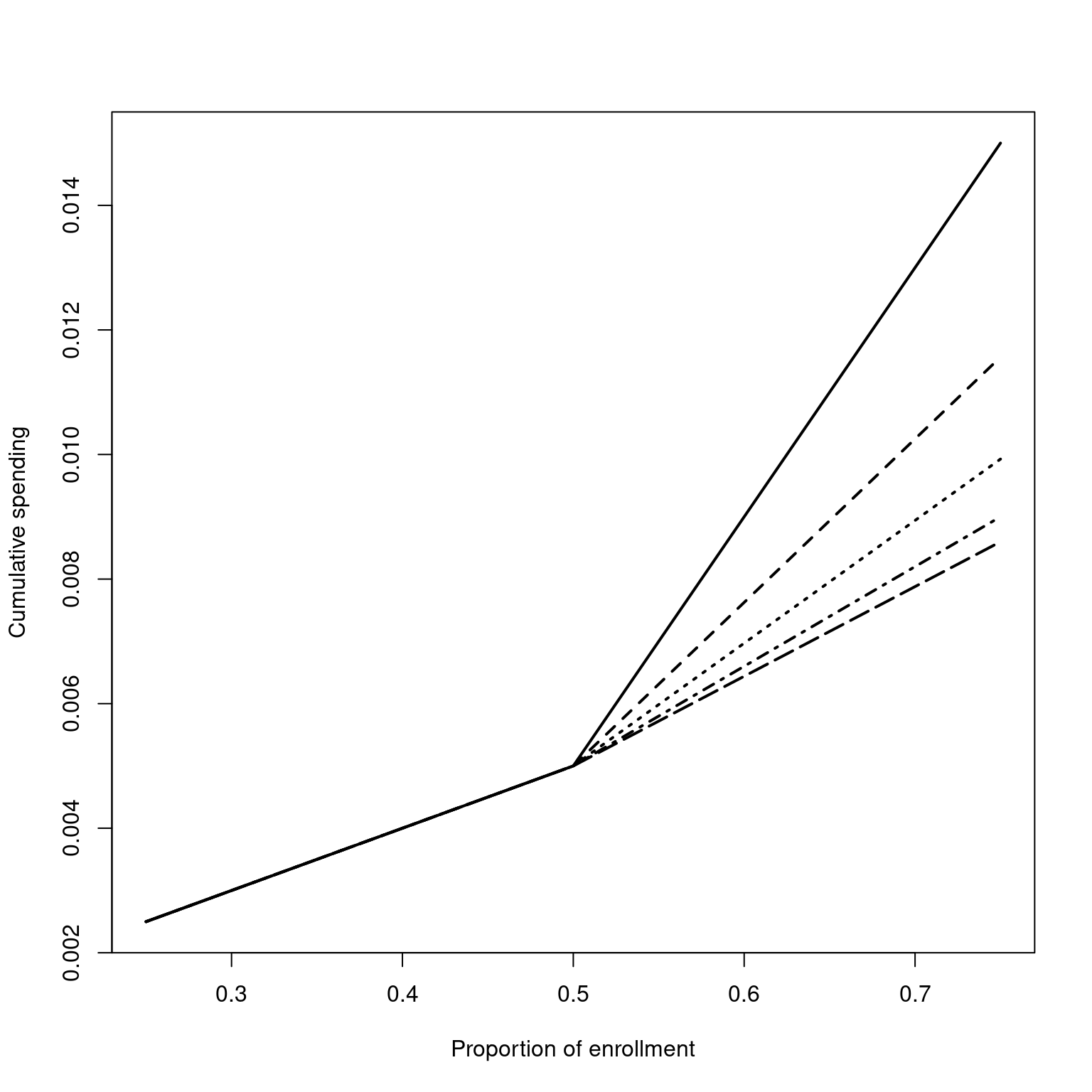

Figure 8.3

8.5.3 Optimized spending functions

The following two examples demonstrate some of the flexibility and research possibilities for the gsDesign package. The particular examples may or may not be of interest, but the strategy may be applied using a variety of optimization criteria. First, we consider finding a spending function to match a Wang-Tsiatis design. This could be useful to adjust a Wang-Tsiatis design if the timing of interim analyses are not as originally planned. Second, we replicate a result from Anderson (Anderson 2007) which minimized expected value of the square of sample size over a family of spending functions and a prior distribution.

8.5.3.1 Approximating a Wang-Tsiatis design

We have noted several approximations of O’Brien-Fleming and Pocock spending rules using spending functions in the table above. Following is sample code to provide a good approximation of Wang-Tsiatis bounds with a given parameter \(\Delta\). This includes O’Brien-Fleming (\(\Delta\)=0) and Pocock (\(\Delta\)=0.5) designs. First, we define a function that computes the sum of squared deviations of the boundaries of a Wang-Tsiatis design compared to a one-parameter spending function family with a given parameter value of x. Note that Delta is the parameter for the Wang-Tsiatis design that we are trying to approximate. Other parameters are as before; recall that test.type should be limited to 1 or 2 for Wang-Tsiatis designs. Defaults are used for parameters for gsDesign() not included here.

WTapprox <- function(
    x,
    alpha = 0.025,
    beta = 0.1,
    k = 3,
    sf = sfHSD,
    Delta = 0.25,
    test.type = 2) {
  # Wang-Tsiatis comparison with a one-parameter spending function
  y1 <- gsDesign(
    k = k,
    alpha = alpha,
    beta = beta,
    test.type = test.type,
    sfu = "WT",
    sfupar = Delta
  )$upper$bound
  y2 <- gsDesign(
    k = k,
    alpha = alpha,
    beta = beta,
    test.type = test.type,
    sfu = sf,
    sfupar = x
  )$upper$bound
  z <- y1 - y2
  return(sum(z * z))
}

We consider approximating a two-sided O’Brien-Fleming design with alpha = 0.025 (one-sided) using the exponential spending function. The function nlminb() is a standard R function used for minimization. It minimizes a function passed to it as a function of that function’s first argument, which may be a vector. The first parameter of nlminb() is a starting value for the minimization routine. The second is the function to be minimized. The parameter lower below provides a lower bound for first argument to the function being passed to nlminb().  Following parameters are fixed parameters for the function being passed to nlminb(). The result suggests that for \(k = 4\), an exponential spending function with \(\nu = 0.75\) approximates an O’Brien-Fleming design well. Examining this same optimization for \(k = 2\) to 10 suggests that \(\nu = 0.75\) provides a good approximation of an O’Brien-Fleming design across this range.

nu <- nlminb(
  start = 0.75,
  objective = WTapprox,
  lower = 0,
  sf = sfExponential,
  k = 4,
  Delta = 0,
  test.type = 2
)$par
nu

Running comparable code for sfHSD() and sfPower() illustrates that the exponential spending function can provide a better approximation of an O’Brien-Fleming design than either the Hwang-Shih-DeCani or Kim-DeMets spending functions. For Pocock designs, the Hwang-Shih-DeCani spending function family provides good approximations.

Minimizing the expected value of a power of sample size

In this example, we first define a function that computes a weighted average across a set of theta values of the expected value of a given power of the sample size for a design. Note that sfupar and sflpar are specified in the first input argument so that they may later be optimized using the R routine nlminb(). The code is compact, which is very nice for writing, but it may be difficult to interpret. A good way to see how the code works is to define values for all of the parameters and run each line from the R command prompt, examining the result.

#' Expected value of the power of sample size of a trial
#' as a function of upper and lower spending parameter.
#' Get sfupar from x[1] and sflpar from x[2].
#'
#' @param val The power of the sample size for which
#'   expected values are computed.
#' @param theta A vector for which expected values
#'   are to be computed.
#' @param thetawgt A vector of the same length used to
#'   compute a weighted average of the expected values.
#'   Other parameters are as for gsDesign.
enasfpar <- function(
    x,
    timing = 1,
    theta,
    thetawgt,
    k = 4,
    test.type = 4,
    alpha = 0.025,
    beta = 0.1,
    astar = 0,
    delta = 0,
    n.fix = 1,
    sfu = sfHSD,
    sfl = sfHSD,
    val = 1,
    tol = 0.000001,
    r = 18) {
  # Derive design
  y <- gsDesign(
    k = k,
    test.type = test.type,
    alpha = alpha,
    beta = beta,
    astar = astar,
    delta = delta,
    n.fix = n.fix,
    timing = timing,
    sfu = sfu,
    sfupar = x[1],
    sfl = sfl,
    sflpar = x[2],
    tol = tol,
    r = r
  )
  # Compute boundary crossing probabilities for input theta
  y <- gsProbability(theta = theta, d = y)
  # Compute sample sizes to the val power
  n <- y$n.I^val
  # Compute expected values
  en <- n %*% (y$upper$prob + y$lower$prob)
  # Compute weighted average of expected values
  en <- sum(as.vector(en) * as.vector(thetawgt))

  return(en)
}

Now we use this function along with the R routine nlminb() which finds a minimum across possible values of sfupar and sflpar. The design derived using the code below and a more extensive discussion can be found in (Anderson 2007). The code above is more general than in (Anderson 2007), however, as that paper was restricted to test.type=5 (the program provided there also worked for test.type=6).

# Example from Anderson (2006)
delta <- abs(qnorm(0.025) + qnorm(0.1))
# Use normal distribution to get weights
x <- normalGrid(mu = delta, sigma = delta / 2)
x <- nlminb(
  start = c(0.7, -0.8),
  enasfpar,
  theta = x$z,
  timing = 1,
  thetawgt = x$wgts,
  val = 2,
  k = 4,
  tol = 0.0000001
)
x$message
y <- gsDesign(
  k = 4,
  test.type = 5,
  sfupar = x$par[1],
  sflpar = x$par[2]
)
y

8.5.4 Writing code for a new spending function

Following is sample code using a cumulative distribution function for a beta-distribution as a spending function. Let B(a,b) denote the complete beta function. The beta distribution spending function is denoted for any fixed \(a>0\) and \(b>0\) by

\[ \alpha(t)=\frac{\alpha}{B(a,b)}% %TCIMACRO{\tint \limits_{0}^{t}}% %BeginExpansion {\textstyle\int\limits_{0}^{t}} %EndExpansion x^{a-1}(1-x)^{b-1}dx. \]

This spending function provides much of the flexibility of spending functions in the last subsection, but is not of the same general form. This sample code is intended to provide guidance in writing code for a new spending function, if needed.

# Implementation of 2-parameter version of beta distribution
# spending function.
# Assumes t and alpha are appropriately specified
# (does not check!).
sfbdist <- function(alpha, t, param) {
  # Set up return list and its class
  x <- list(
    name = "B-dist example",
    param = param,
    parname = c("a", "b"),
    sf = sfbdist,
    spend = NULL,
    bound = NULL,
    prob = NULL,
    errcode = 0,
    errmsg = "No error"
  )
  class(x) <- "spendfn"
  # Check for errors in specification of a and b
  # gsReturnError is a simple function available from the
  # package for saving errors in the returned value
  if (length(param) != 2) {
    return(gsReturnError(x,
      errcode = 0.3,
      errmsg = "b-dist example spending function parameter must be of length 2"
    ))
  }
  if (!is.numeric(param)) {
    return(gsReturnError(x,
      errcode = 0.1,
      errmsg = "Beta distribution spending function parameter must be numeric"
    ))
  }
  if (param[1] <= 0) {
    return(gsReturnError(x,
      errcode = 0.12,
      errmsg = "1st Beta distribution spending function parameter must be > 0."
    ))
  }
  if (param[2] <= 0) {
    return(gsReturnError(x,
      errcode = 0.13,
      errmsg = "2nd Beta distribution spending function parameter must be > 0."
    ))
  }
  # Set spending using cumulative beta distribution function and return
  x$spend <- alpha * pbeta(t, x$param[1], x$param[2])
  return(x)
}

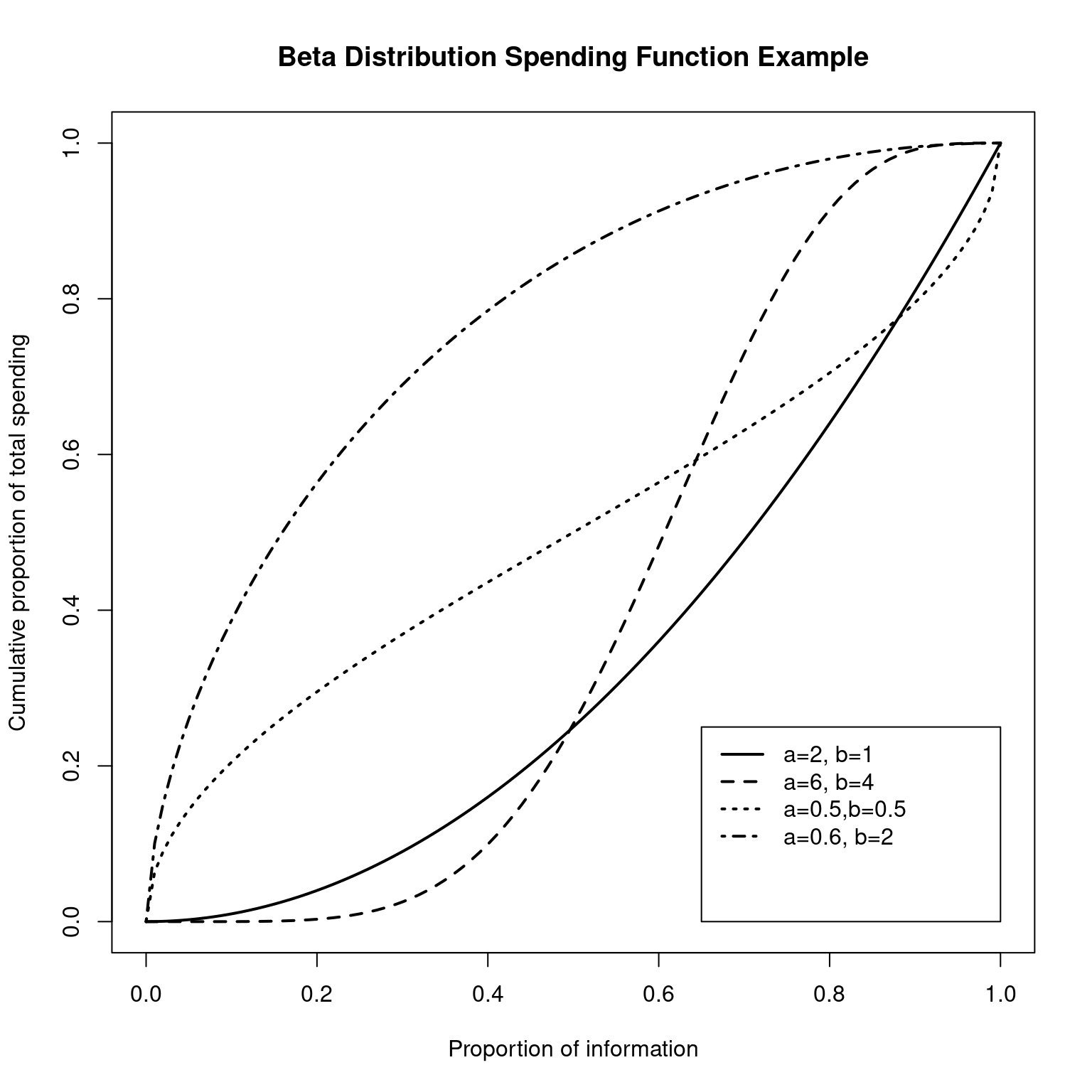
The flexibility of this spending function is demonstrated by the following code which produces the plot below. Using a = \(\rho\), b = 1 produces a Kim-DeMets spending function \(\alpha t^{\rho}\) as shown by the solid line with \(\rho\)=2. The dashed line (a = 6, b = 4) shows a spending function that is conservative very early, but then aggressive in its spending pattern starting after about 40% of data are available. The dotted (a = 0.5, b = 0.5) and dot-dashed (a = 0.6, b = 2) show increasingly aggressive early spending. These may be useful in setting an initial high futility bound when the first part of a trial is used as a proof of concept for a clinical endpoint.

# Plot some beta distribution spending functions
plot(0:100 / 100, sfbdist(1, 0:100 / 100, c(2, 1))$spend,
  type = "l", lwd = 2,
  xlab = "Proportion of information",
  ylab = "Cumulative proportion of total spending",
  main = "Beta Distribution Spending Function Example"
)
lines(
  0:100 / 100, sfbdist(1, 0:100 / 100, c(6, 4))$spend,
  lty = 2, lwd = 2
)
lines(
  0:100 / 100, sfbdist(1, 0:100 / 100, c(0.5, 0.5))$spend,
  lty = 3, lwd = 2
)
lines(
  0:100 / 100, sfbdist(1, 0:100 / 100, c(0.6, 2))$spend,
  lty = 4, lwd = 2
)
legend(
  x = c(0.65, 1), y = 1 * c(0, 0.25), lty = 1:4, lwd = 2,
  legend = c(
    "a=2, b=1", "a=6, b=4", "a=0.5,b=0.5", "a=0.6, b=2"
  )
)

Figure 8.4

Anderson, Keaven M. 2007. “Optimal Spending Functions for Asymmetric Group Sequential Designs.” Biometrical Journal 49 (3): 337–45.

Hwang, Irving K, Weichung J Shih, and John S De Cani. 1990. “Group Sequential Designs Using a Family of Type 1 Error Probability Spending Functions.” Statistics in Medicine 9 (12): 1439–45.

Jennison, Christopher, and Bruce W. Turnbull. 2000. Group Sequential Methods with Applications to Clinical Trials. Boca Raton, FL: Chapman; Hall/CRC.

Lan, K K Gordon, and David L DeMets. 1983. “Discrete Sequential Boundaries for Clinical Trials.” Biometrika 70 (3): 659–63.

The CAPTURE Investigators. 1997. “Randomised Placebo-Controlled Trial of Abciximab Before and During Coronary Intervention in Refractory Unstable Angina: The CAPTURE Study.” The Lancet 349 (9063): 1429–35.

The GUSTO V Investigators. 2001. “Reperfusion Therapy for Acute Myocardial Infarction with Fibrinolytic Therapy or Combination Reduced Fibrinolytic Therapy and Platelet Glycoprotein IIb/IIIa Inhibition: The GUSTO V Randomised Trial.” The Lancet 357 (9272): 1905–14.