[1] 0.00345 More time-to-event design
We consider variations on time-to-event designs that come up from time-to-time. The mainstream approaches are given in the previous chapter. Here we give more design examples. We consider in greater detail:
- Fixed enrollment rates with variable follow-up duration.
- Variable enrollment duration with a fixed enrollment rate and minimum follow-up duration.
- Calendar-based timing of analyses and calendar-based spending bounds.
- Fixed duration of follow-up on a per patient basis.
Other than calendar-based design, these can produce some numerical challenges which arise with some frequency. We provide examples and how to work around these challenges.
5.1 Fixed enrollment rates, variable follow-up duration
It may be operationally impossible to enroll more than a certain number of patients per month and also may be desirable to limit total enrollment. We present a cardiovascular endpoint study to demonstrate considerations. For this, we assume a control group event rate of 4% per year. To translate this to a monthly exponential failure rate, we compute
In Figure 5.1, we specify this as well as an exponential dropout rate of 0.001 which corresponds to an annual dropout rate of
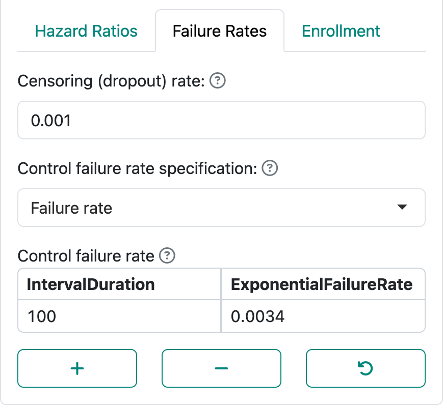
As in many of our examples, we set timing of analyses after 35% and 70% of statistical information, which is equivalent to 35% and 70% of the final targeted events. In this case, we have selected 85% power for a hazard ratio of 0.8.
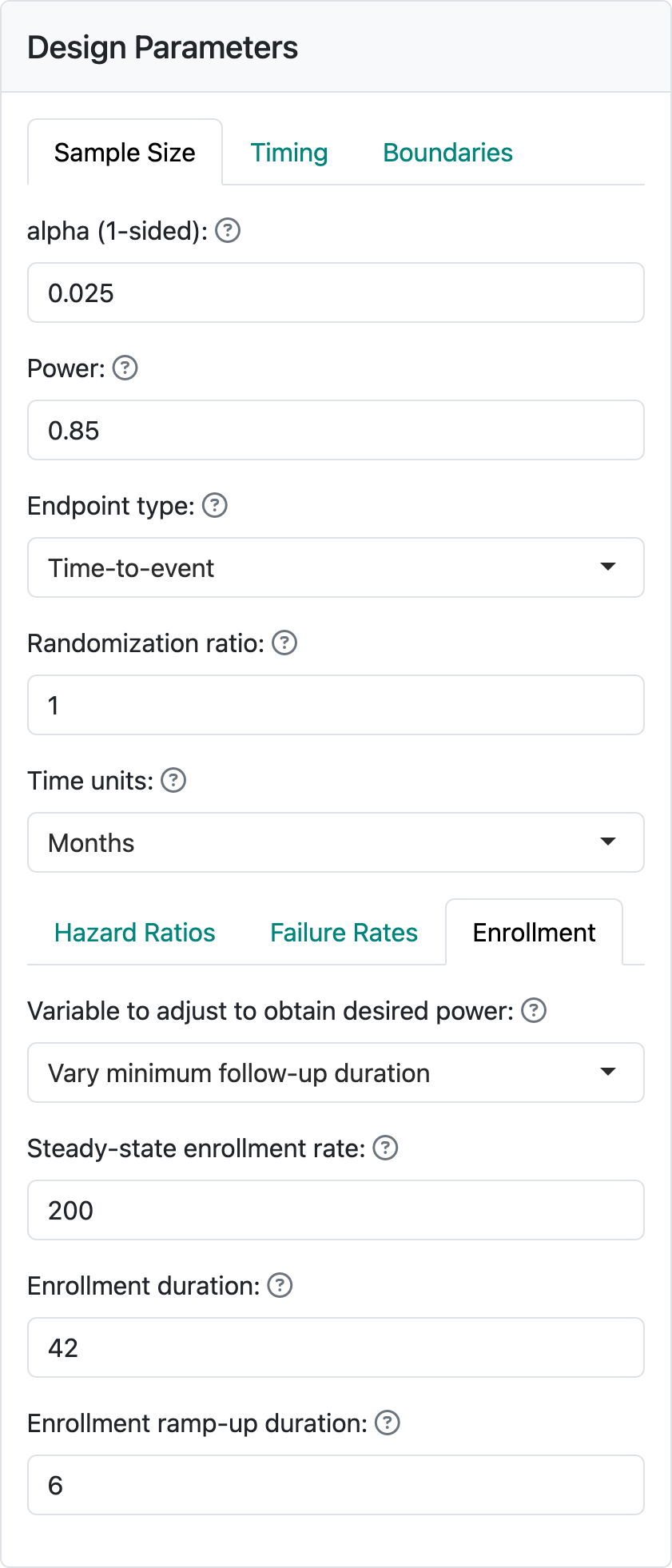
We have set a maximum enrollment of 200 participants per month and a targeted enrollment duration of 42 months, as seen in Figure 5.2.
For the bounds, we have used a Lan-DeMets spending function used to approximate O’Brien-Fleming bounds. This is a commonly recommended spending function by regulators and is generally widely accepted. For futility, we use a bespoke (custom) \(\beta\)-spending (Anderson and Clark 2010) that specifies targeted \(\beta\)-spending at 2 points of statistical information. This is done by selecting the 2-parameter spending function option. In this case we have selected a Cauchy spending function, but the other choices fit the same 2 spending points with different distribution shapes, as shown in Figure 5.3. In this case, we chose 20% of \(\beta\)-spending after 35% of statistical information to require approximately a hazard ratio of > 1 to cross the bound; this would suggest the sponsor may wish to discontinue the trial without at least a minimal positive trend in favor of the control group. Since chronic treatment of, say, cholesterol may not result in an immediate benefit, this fairly weak futility bound may be appropriate. At the second interim, we set 50% of cumulative \(\beta\)-spending which corresponds to an observed hazard ratio of approximately 0.91. These choices can be worked through and customized with discussions with regulators and the design team for the study. Recall that we are using the default of non-binding futility bounds which means that Type I error is controlled whether or not a trial is stopped after crossing a futility bound.
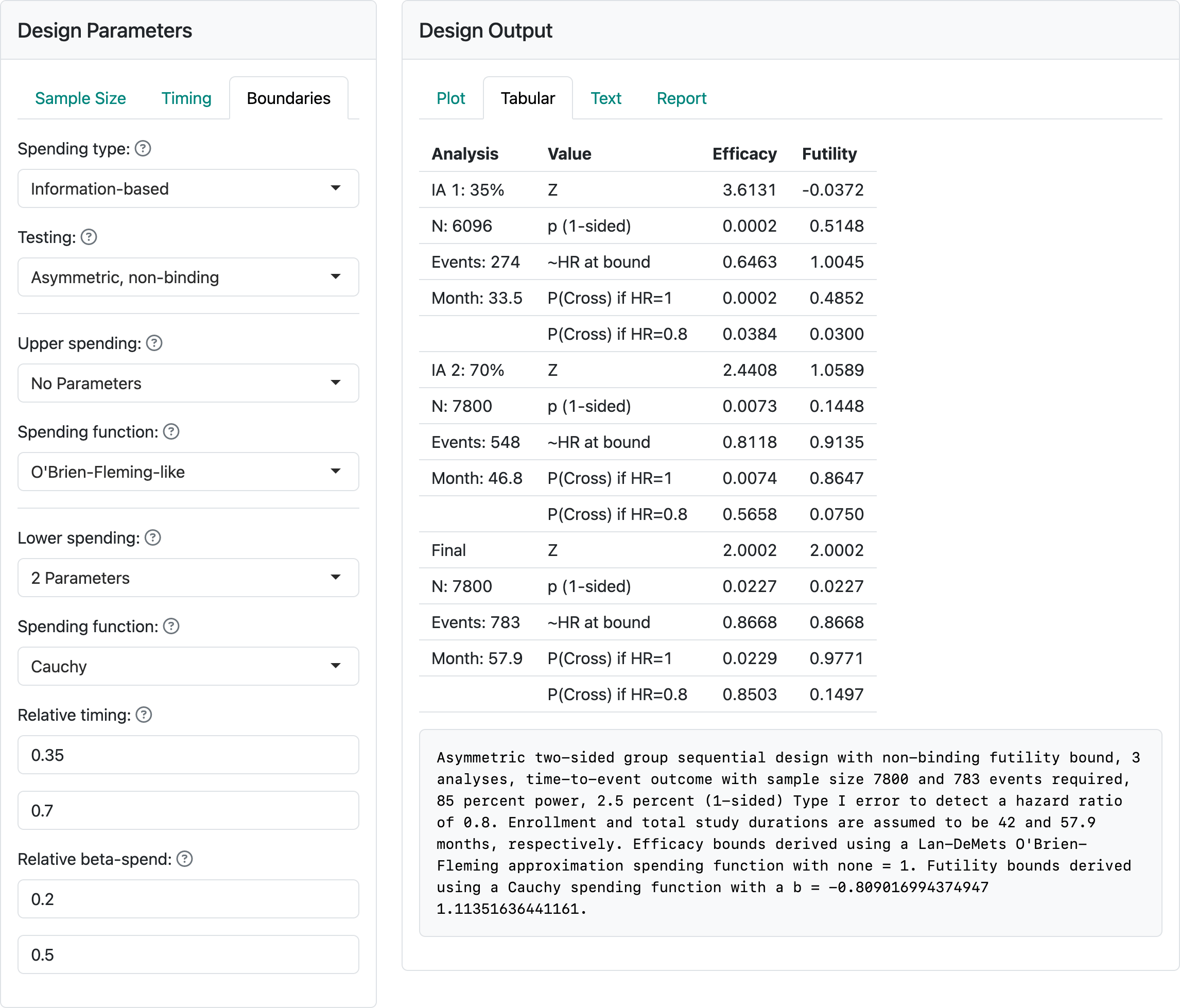
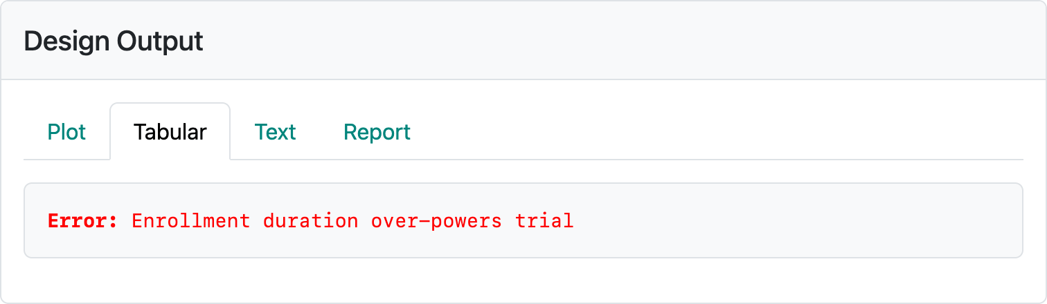
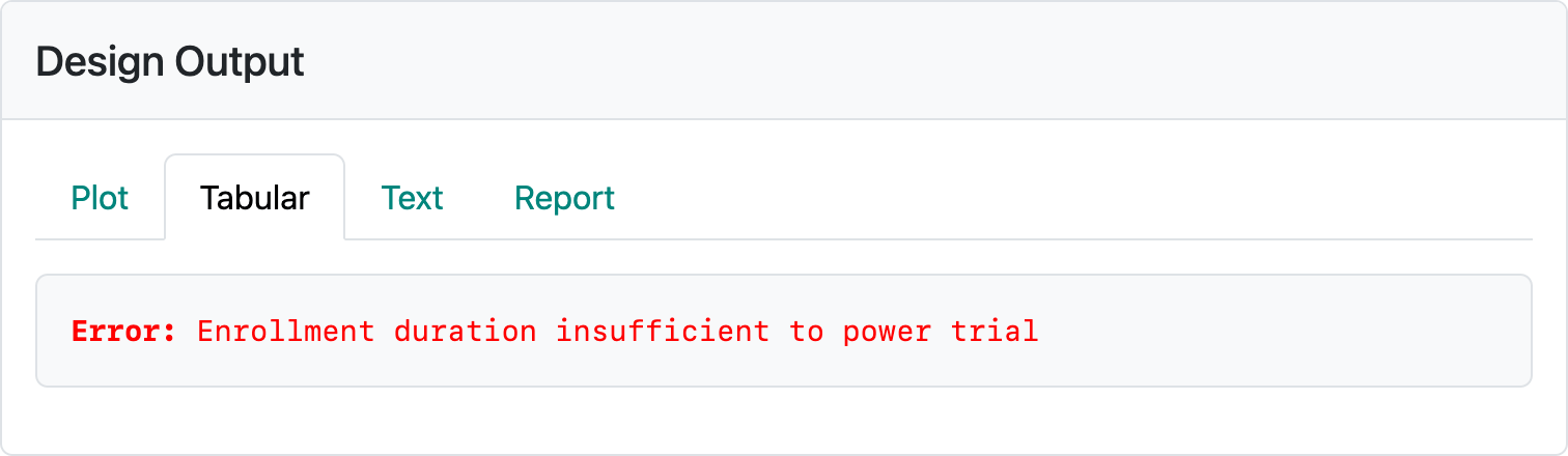
The above design requires about 58 months to complete if the design assumptions are correct. If event rates are higher or lower, expected trial duration will be shorter or longer, respectively. If you restore this design from vary-minimum-follow-up-design.rds and change the number of participants enrolled per month, you can see some of the challenges of this method. If 400 is entered for the enrollment per month, the error message in Figure 5.4 occurs.
If enrollment rates are too low, the trial can be too long; e.g., 100 per month results in an expected trial duration of 99 months. Entering 20 per month enrollment results in the error displayed in Figure 5.5.
5.2 Vary enrollment duration, fix enrollment rate and follow-up duration
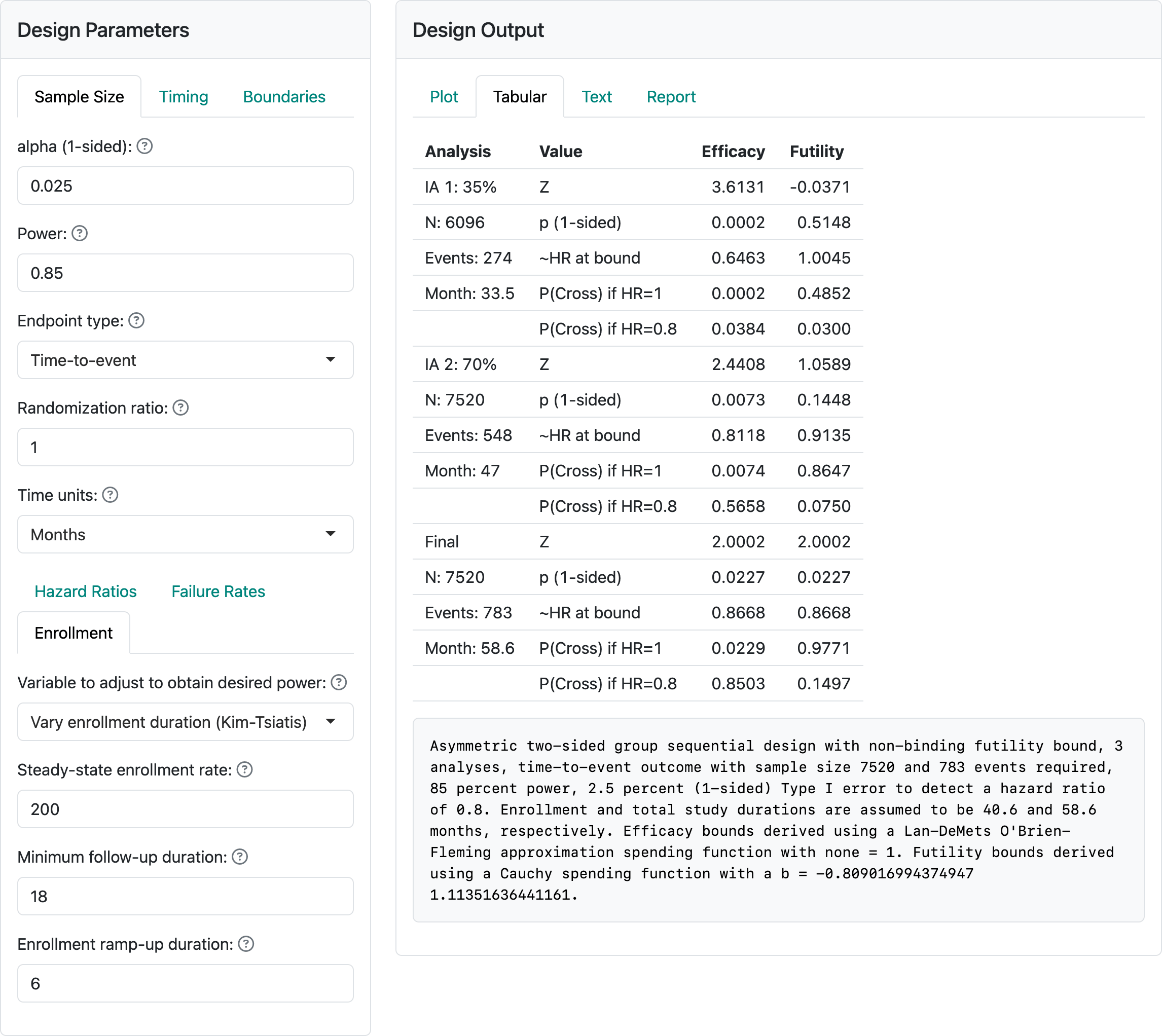
Kim and Tsiatis (1990) provided a sample size method where enrollment rate is fixed as above and minimum follow-up duration is also fixed. This method varies the enrollment duration and, thus, sample size to achieve the targeted power. We continue the example from the previous section. In this case, we specify a minimum follow-up and let the enrollment duration vary. As shown in Figure 5.6, this results in a slightly smaller sample size for this case (7520 below vs. 7800 above) with little difference in expected trial duration (58.6 months below vs. 57.9 months above).
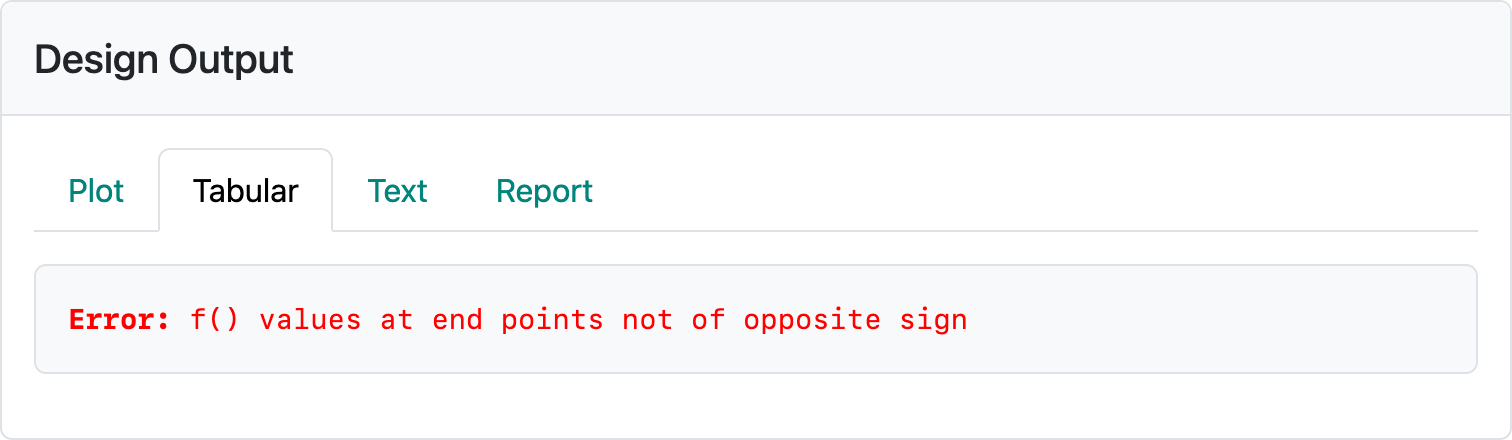
The Kim and Tsiatis (1990) method is much less susceptible to the types of errors we could easily generate above. However, with an enrollment of 700 per month, we get the error in Figure 5.7.
It is still easy to get trial durations that are unattractive if enrollment rates are limited.
5.3 Calendar-based timing and spending with cure model
For trials with low-risk cancers such as previously untreated patients undergoing surgery to remove a tumor with study add-on therapy to reduce disease recurrence there can be a very good chance of long-term remission of disease. Among those with recurrence, it can happen early in the course of follow-up. This can be modeled reasonably well with piecewise exponential rates if the user desires. A cure model presented by Rodrigues et al. (2009) has been built into the gsDesign Shiny interface. Whether or not you believe in cured patients, this provides a simple way to design when failure rates are expected to decrease over time. Whichever approach you choose to approximate a scenario with decreasing event rates over time, we suggest calendar-based spending (Lan and DeMets 1989) as a possible consideration. We present some strategies on how to do this effectively.
The Poisson mixture model assumes a cure rate \(p\) to represent the patients who benefit long-term. The survival function as a function of time \(t\) for a control group (\(c\)) is:
\[S_c(t)=\exp(-\theta(1-\exp(-\lambda t))),\] where \(\theta = -\log(p)\), \(\lambda> 0\) is a constant hazard rate and \(t \geq 0\). We note that under a proportional hazards assumption with hazard ratio \(\gamma > 0\) the survival function for the experimental group (e) still fits the Poisson mixture model:
\[S_e(t)=\exp(-\theta\gamma(1-\exp(-\lambda t))).\] For any setting chosen, it is ideal to be able to cite published literature and other rationale for study assumptions and show that the Poisson mixture assumptions for the control group reasonably match historical data.
The component \(\exp(-\lambda t)\) above is an exponential survival distribution. This two-parameter model for the control group can be specified by the cure rate and the assumed survival rate \(S_c(t_1)\) at some time \(0 <t_1<\infty.\) We see this specification in Figure 5.8.
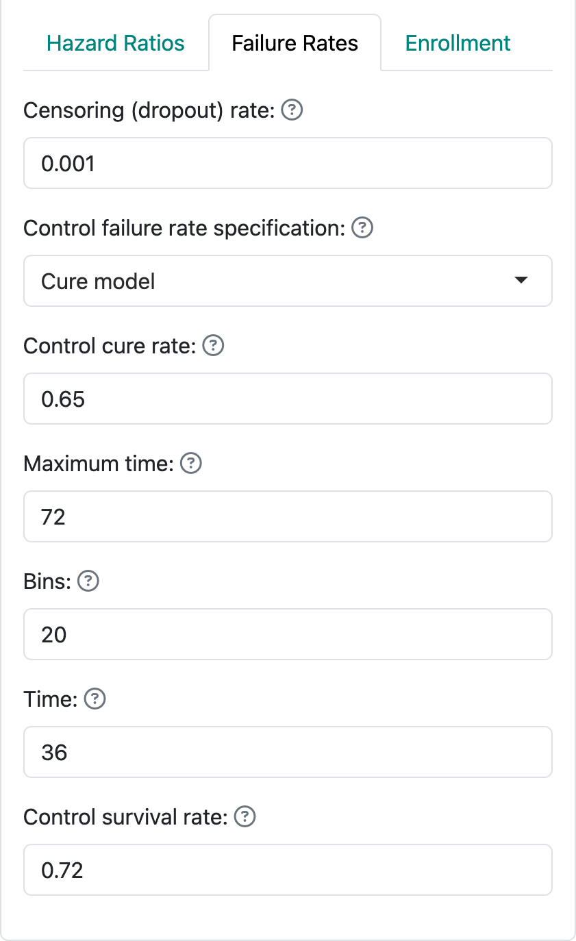
We have specified a cure rate \(p=0.65\) and a survival rate of \(S_c(36) = 0.72\) for the control group. For this example we power the trial at 90% for a hazard ratio of 0.76 with one-sided Type I error of 2.5%. This implies an experimental group cure rate of
\[0.65^{0.76} = 0.72\]
The maximum time in Figure 5.8 is not for trial duration; it is specifying an end to the window where piecewise exponential rates over intervals will be used to approximate the Poisson mixture survival distribution. Trial duration is specified as before, in this case with enrollment duration plus minimum follow-up used with the Lachin-Foulkes method for sample size derivation. To see this design, restore it from calendar-based-design-with-cure.rds.
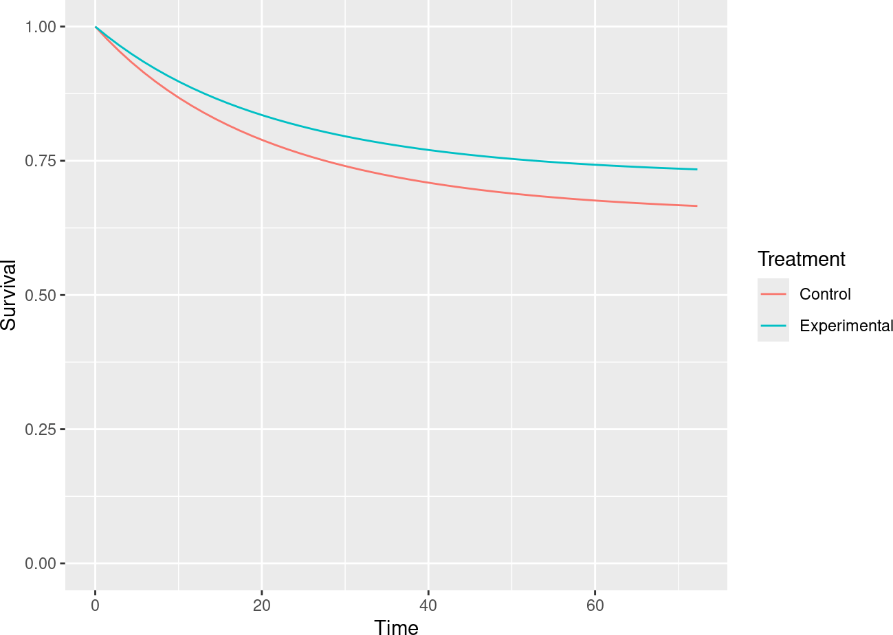
We specify that timing of analyses is calendar-driven rather than event-driven. The underlying survival curves can be viewed by scrolling to the bottom of the Report tab and downloading the html version of the report or by downloading the .Rmd version and running it to generate the report documenting the design. In the report, you will see the underlying survival curves in Figure 5.9 for the control and experimental treatment groups. Note the flattening tail the reflects the decreasing late disease recurrence rates.
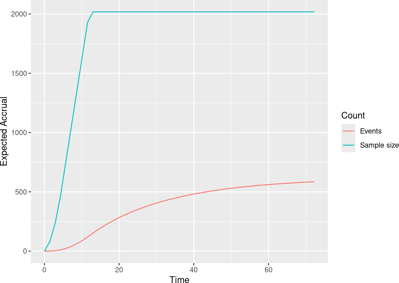
This results in a slowing expected accumulation of events as can be seen in another plot (Figure 5.10) from the same report.
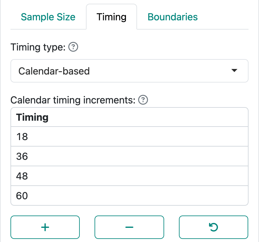
It is convenient for designs with changing failure rates that may be hard to anticipate to do initial planning of analyses using calendar time rather than information fraction as we have done previously. Figure 5.11 demonstrates how this is done from the Timing input tab.
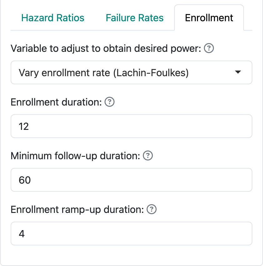
As noted in this graphic, you need to specify study duration in the Enrollment input tab. Here we specify 12-month enrollment duration with a minimum of 60 months of follow-up; together, these specify a total study duration of 72 months (Figure 5.12).
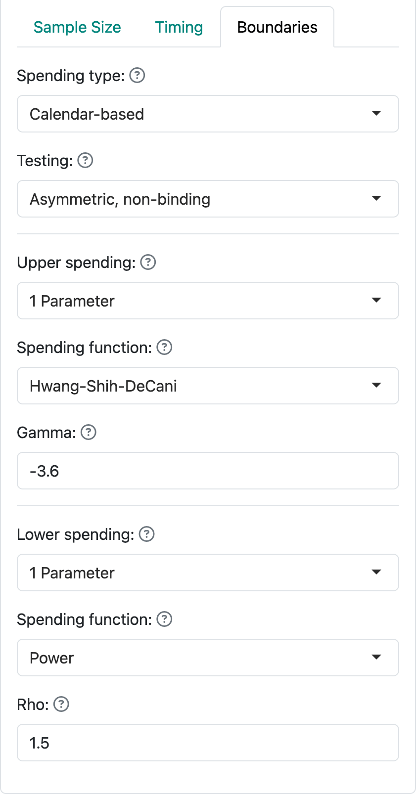
For this case, we also specify calendar-based spending (Lan and DeMets 1989) as shown in Figure 5.13.
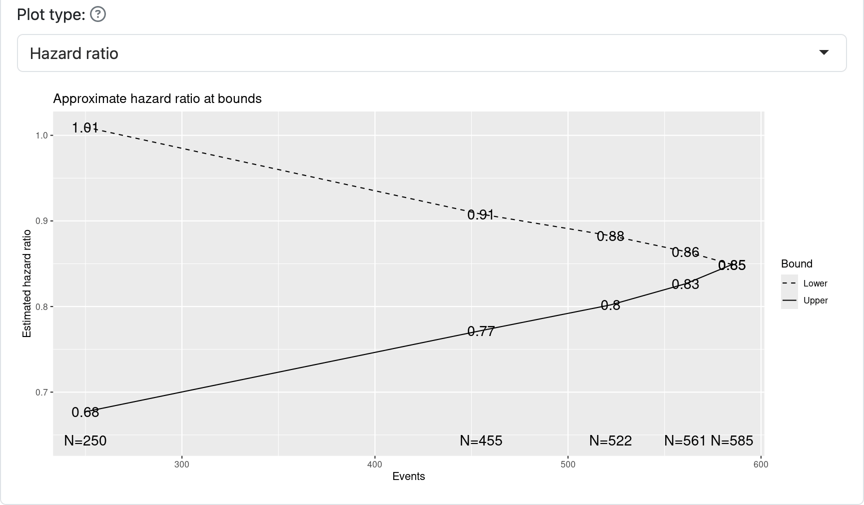
All of the above results in the following design as summarized in Figure 5.14 by using approximate hazard ratio values required to cross efficacy and futility bounds.
It will be important to specify in a corresponding protocol when the interim and final analyses will be done. For this case, we will assume all is calendar-based according to plan and any shortfall or excess of events will result in a corresponding decrease or increase of events. For instance, by changing the power to 80% and leaving other parameters the same we see that 434 events yields 80% power instead of the planned 90% power with 585 events, both with the underlying assumption of a hazard ratio of 0.76 for experimental treatment versus control. Alternatively, changing the targeted hazard ratio to 0.73 yields a requirement of 445 events. The trial sponsor has to decide if these tradeoffs are acceptable and presumably get buy-in from regulators.
Because of the slow accumulation of events late in the trial, the expected statistical information under design assumptions is very close to the final information at the final interim (96%). With information-based spending, this can result in very little spending left for the final analysis, thus providing some potential advantage for calendar-based spending. On the other hand, spending can be much less for some interim analyses with calendar-based spending if the same spending functions are used for calendar- and information-based design. Thus, the choice of spending functions is critical; to convince regulators and your team that this design is worth considering will involve comparing the design to a more conventional spending function with information-based spending. For the design chosen, an O’Brien-Fleming-like spending function with information-based spending requires a final nominal \(p\)-value substantially smaller than what we have here at the final analysis.
5.3.1 Updating bounds when using calendar-based spending
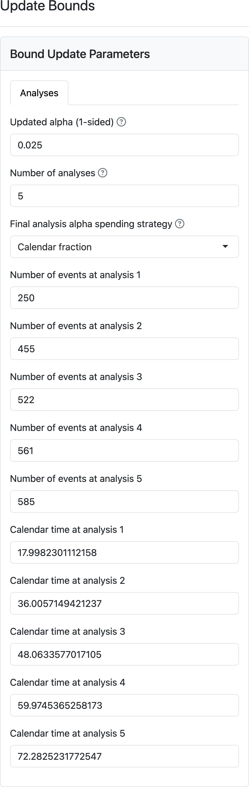
Updating a design with calendar-based spending requires both the events available at each analysis as well as the calendar time of the analysis relative to the start of the trial. The event counts determine the asymptotic multivariate normal distribution that is used with group sequential design to approximate boundary crossing probabilities. The calendar times of analyses determine the cumulative amount of alpha- and beta-spending for each analysis. Below is the interface for updating analyses. As before, you are allowed to modify the total alpha and the number of analyses. Also as before, you specify the number of events at each analysis. Because the default of integer-based design was used, event counts from the design shown in Figure 5.15 are all integers. On the other hand, the calendar timing of achieving these targeted events from the design was altered from the input slightly to ensure integer-based event counts in the design.
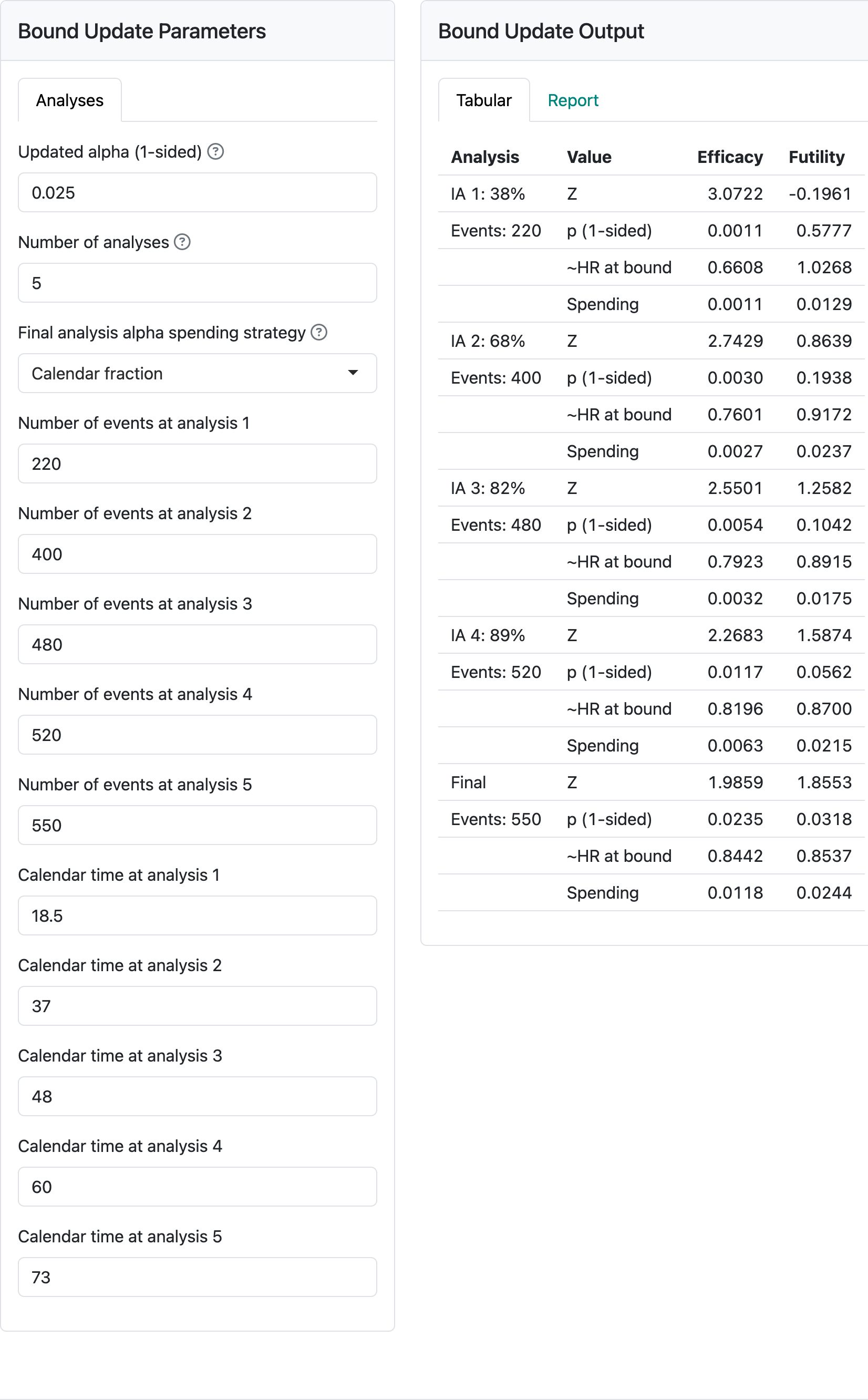
Now we update the calendar timing and event counts to see the impact on bounds in Figure Figure 5.16. Note that the full alpha is spent at the final analysis even given the shortfall of events at the final analysis (580 targeted, 550 observed). The cumulative probability of crossing the efficacy bound of 0.0235 is due to the standard choice of a non-binding futility bound rather than a shortfall in spending; adding the numbers under spending for the efficacy bound will total 0.025. This ensures a nominal \(p\)-value that is fairly close to 0.025 for the final analysis whether events accrue more slowly or faster than anticipated in the design. The shortfall of events in Figure 5.16 will have a small impact on power, but that is likely outweighed by the apparent need to follow study participants than more than another year to achieve the targeted events. If shortfalls are much more substantial, the tradeoff of longer follow-up of more enrollment might be considered through a protocol amendment. If events occur at faster than targeted rates, power will be greater than targeted. However, no amendment may be desired as the final follow-up will provide good supportive analyses for things like observed survival differences in a landmark time point such as 5 or 6 years.
5.4 Fixed-follow-up time-to-event outcome
We consider a trial where there is a fixed amount of follow-up planned for each participant enrolled. After this fixed follow-up period, events do not count in the primary analysis. This may be useful when the treatment duration is limited and there is no reasonable expectation that late event rates are impacted by experimental treatment after the specified follow-up time period. For our example, we will assume 24 months of follow-up is used. That is, if a person has an event at 25 months after start of treatment, this event will not count in the primary analysis.
The fixed follow-up period is entered in the failure rate table as shown in Figure 5.17. Here we assume an exponential dropout rate of 0.01 per month and a exponential control failure rate of 0.008 per month.
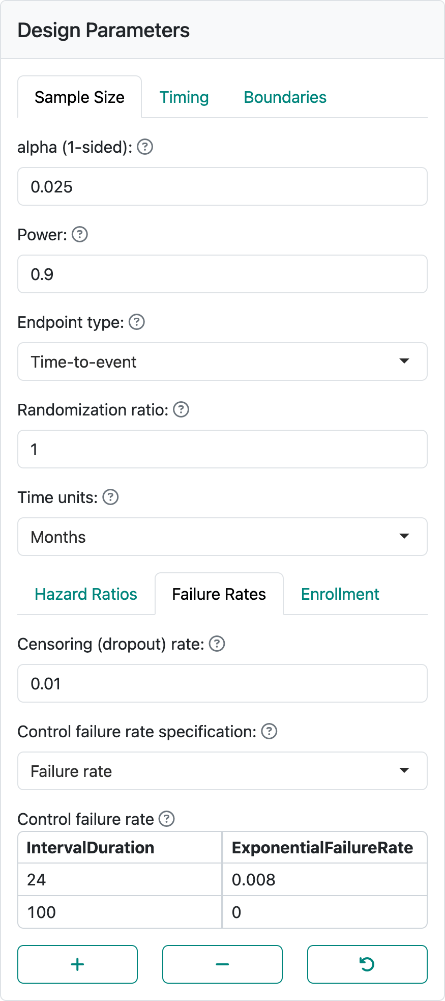
In the enrollment tab, we select the Lachin-Foulkes method. We set the enrollment duration to 12 months, the minimum follow-up duration to 24 months, and the enrollment ramp-up duration to 0 months. We have used the same timing, same alpha, power, interim analysis timing, and spending functions as the example design in Chapter 4.
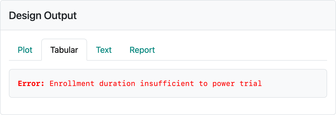
If we have the default of integer-based sample size and event counts, we see the error in Figure 5.18.
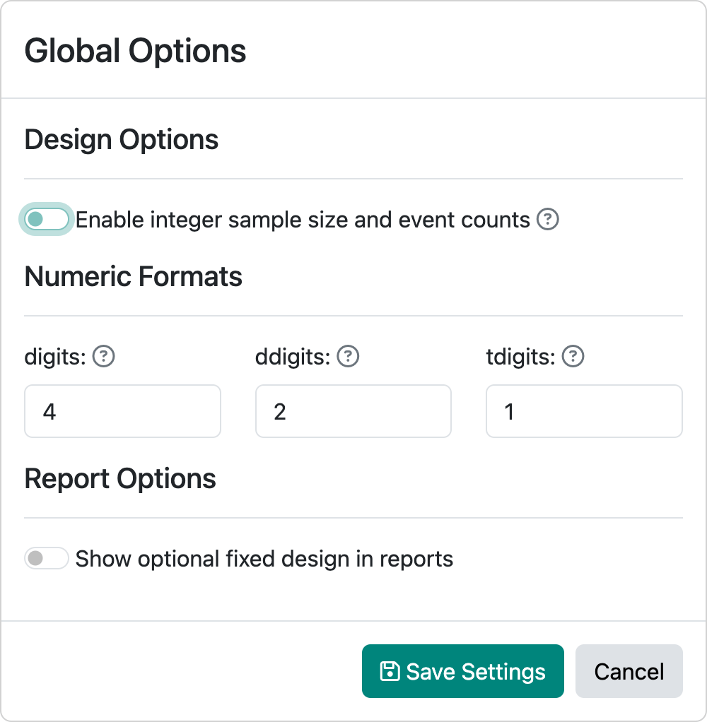
This can be corrected by turning off the integer-based sample size in the global options in Figure 5.19.
This results in the design shown in Figure 5.20.
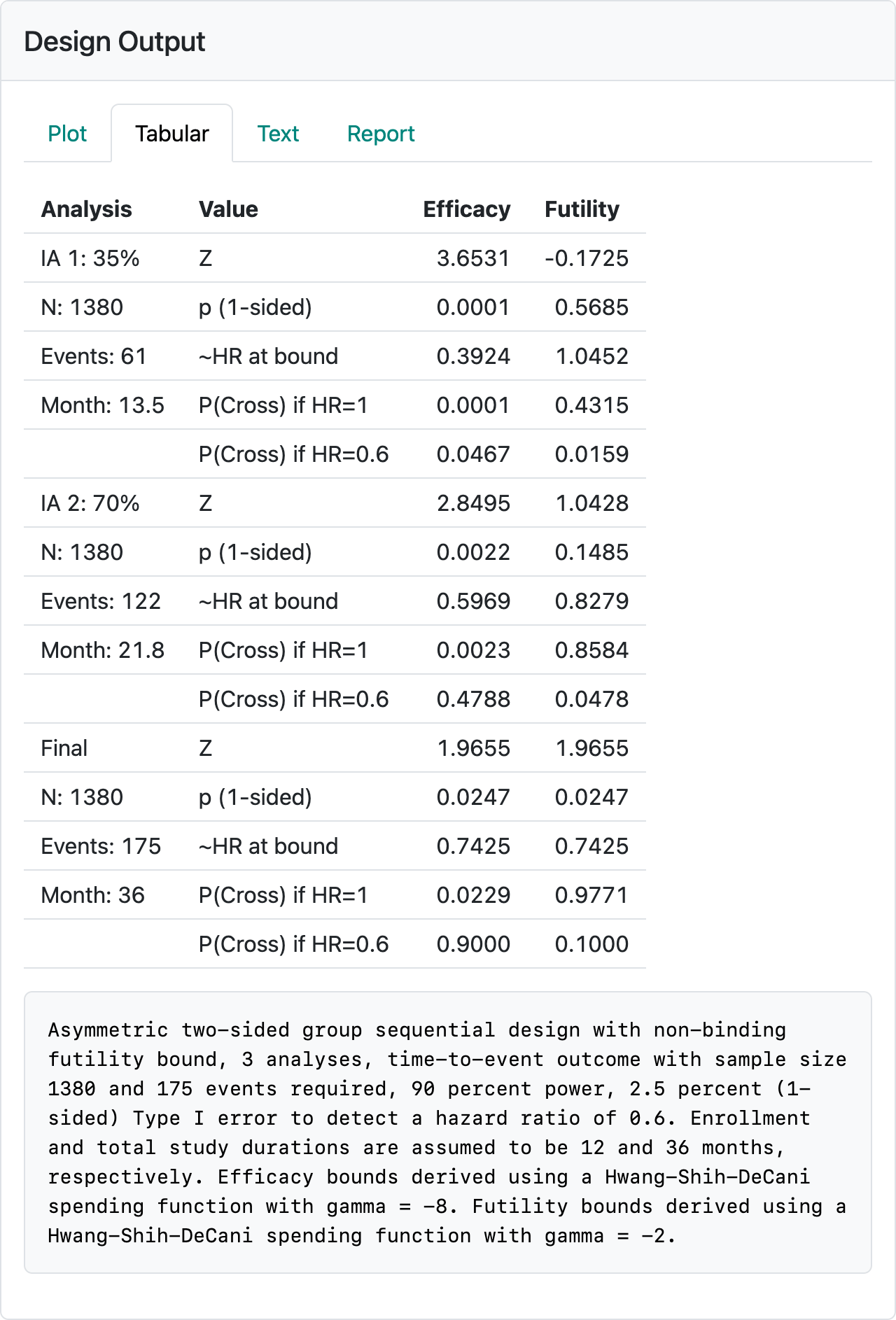
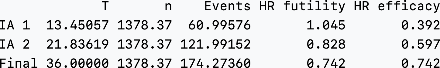
Selecting the “Text” tab and looking near the bottom of the output, we see that under the column n we have a non-integer sample size of 1378.37 and a non-integer Events with a final event count of 174.27 (Figure 5.21).
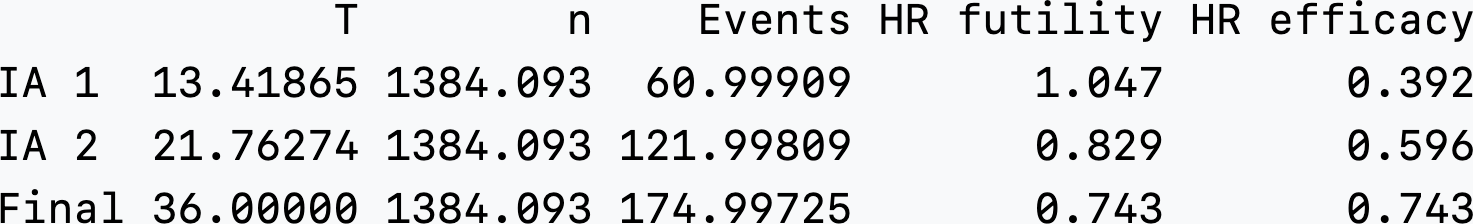
We can manually adjust the power to 0.90124 and interim fractions to 61/175 = 0.3485717 and 122/175 = 0.6971429 to get approximate integer event counts at both interim and final analyses as well as. This strategy targeted 175 final events by increasing power and by setting interim timing to be at 61 and 122 events based on the non-integer design above. In Figure 5.22, there is still not an integer-based sample size (n = 1384.093). This will have the advantage of making the interim spending unambiguous since the denominator for event fractions used for spending is set to essentially 175 regardless of whether the design value (174.997) or rounded value (175) is used; i.e., we should have accuracy for 5 digits.
In actuality, the final event count will be a random number and that if the design control failure rate or hazard ratio does not reflect reality, final event counts can be quite different from 175. Normally, this would be dealt with by increasing follow-up. However, since follow-up is fixed by design for this case, this is not possible. Any correction in sample size to adapt this design would have to be done before the targeted enrollment were reached and could be done using blinded overall event rates and dropout rates. To approximate the average hazard rate the total events observed divided by the total follow-up time summed across study participants could be used. To approximate the dropout rate, the total dropouts divided by the total follow-up time could be used.