8 Spending functions
The gsDesign web interface sets interim boundaries using spending functions. The capabilities allow a great deal of flexibility. We discuss these capabilities and the tradeoffs of different approaches.
8.1 Overview and definition
Spending functions allow flexibility when the timing or number of interim analyses changes during the course of a trial. This will be demonstrated further in Chapter 9. Here we discuss how to choose spending functions at the time of design. We begin with spending functions without parameters, one of which is frequently used. This is followed by one-parameter spending functions that provide additional flexibility and discuss when that flexibility may be desirable. The ultimate flexibility is supplied by piecewise-linear spending functions, which are explained next. We end with 2- and 3-parameter spending functions that also provide increased flexibility over single-parameter spending functions.
The CAPTURE trial (The CAPTURE Investigators 1997) was one of the first trials designed by one of the co-authors (KA) of this book. The statistician for the data monitoring committee was Jan Tijssen from the Academic Medical Center in Amsterdam. Professor Tijssen’s thoughts influenced the CAPTURE trial design as well as the thoughts behind several subsequent trials. The basic philosophy suggested is:
- Set the timing of interim analyses so that the analyses are relevant. That is, do they come at distinct times where it could be reasonable to make decisions.
- Set the efficacy bounds so that they are stringent both from a Type I error perspective and if the trial is stopped, the treatment effect observed is likely to be clinically significant.
- Set futility bounds so that a trial is not stopped too soon (Type II error), but also see if the approximate treatment effect at the futility bound is poor enough that it would not encourage continuing the trial. Also, the timing must be relevant in that substantial time or savings (in terms of patient enrollment and/or costs) is achieved or patients are spared potentially toxic and/or inefficacious treatment.
These thoughts are expressed more fully in an article by Anderson and Clark (2010), and we try to reflect them also here. Since the software specifically estimates the number of patients enrolled at analysis cutoff dates corresponding to achieving a specified number of events for time-to-event endpoints, we focus on such designs here. Note that if there is a substantial gap between the data cutoff and when a decision may be made based on an interim analysis, then enrollment when the trial is stopped may be substantially larger than stated here. This should be considered when selecting a design.
In the following, we continue the example from Chapter 2 where we began with a fixed design sample size of 100 and powered the trial to detect a treatment effect of \(\delta = 5\).
Spending functions are non-decreasing (usually increasing and continuous) functions that are used to select the probability of crossing each interim boundary having not previously crossed a bound. A Type I error spending functions \(f(t)\) is defined for \(0 \leq t\) and with \(f(t) = \alpha\) for \(t \geq 1\). Analogously, a Type II error spending function \(g(t)\) is defined for \(0 \leq t\) and has \(g(t) = \beta\), the Type II error (one minus the power) for \(t \geq 1\). For normal or binomial endpoints, \(t\) represents the proportion of the final planned sample size included at the time of an analysis. For a time-to-event endpoint, \(t\) represents the proportion of the final planned number of events included at the time of an analysis; and alternative for this case is the proportion of planned calendar time for a trial that has passed at the time of data cutoff. For information-based design, \(t\) represents the proportion of the final planned statistical information at the time of an analysis. We let \(t_i\) represent the proportion of total sample size at analysis \(i\) where \(i = 1, 2, 3\) in this case. For information-based spending, we have provided the option for \(t\) to represent the minimum of planned and actual information fraction at each analysis. For both information- and calendar-based spending, we have provided the option of setting \(t=1\) at the final analysis if there is underrunning of the planned final time or information. The actual probability of first crossing an efficacy bound at analysis \(i\) under the null hypothesis is \(f (t_i) - f (t_{i-1})\) where \(t_0 = 0\). The probability of first crossing a futility bound at analysis \(i\) is \(g(t_i) - g(t_{i-1})\). For those interested in more mathematical detail, the books by Jennison and Turnbull (2000) or Proschan et al. (2006) provide nice introductions.
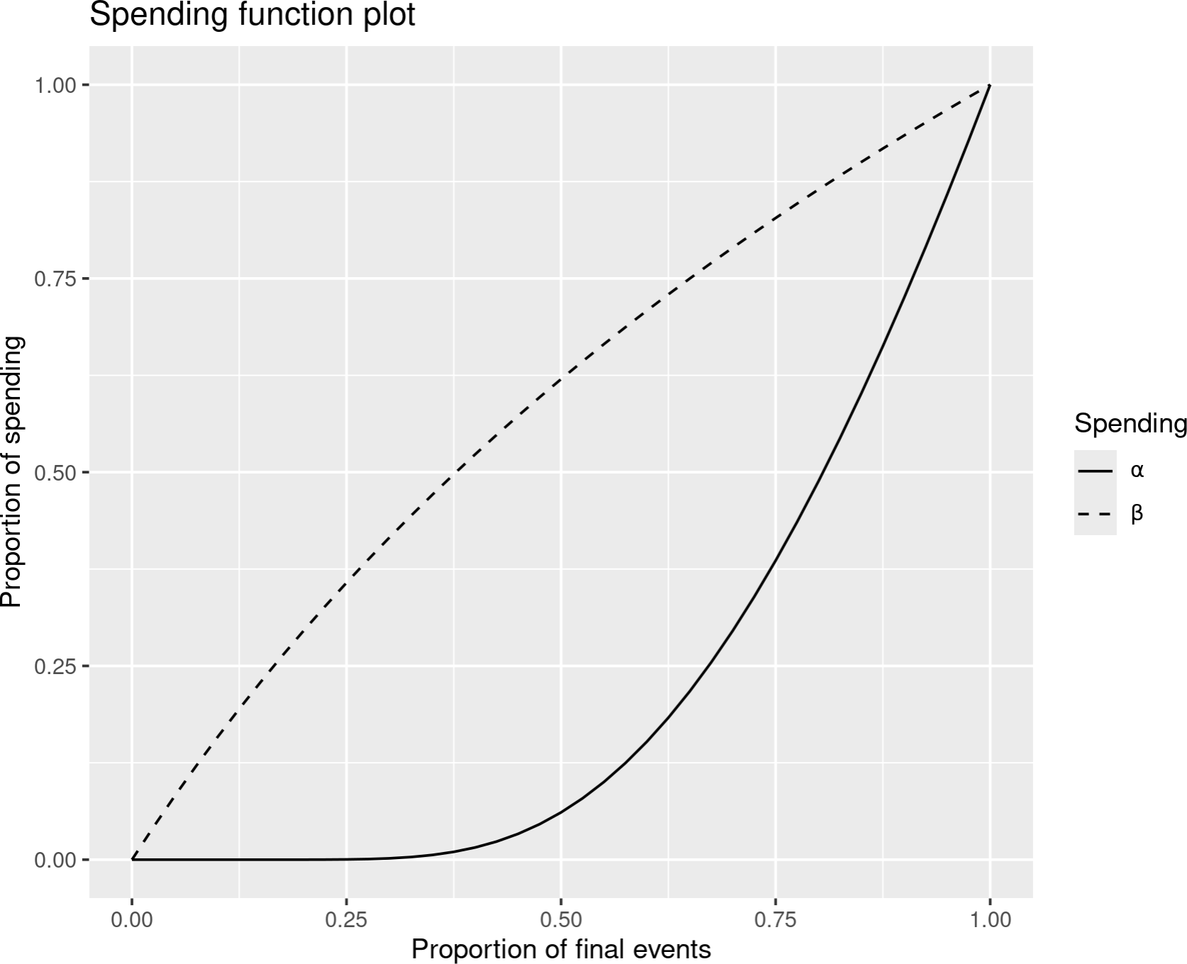
The web interface provides a spending function plot. In Figure 8.1, you see an example using O’Brien-Fleming-like spending function for efficacy (solid line) and Pocock-like spending function for futility (dashed line) as described in the next two sections. Starting from the design in Chapter 2, you can get this plot by using the “Boundaries” tab. Change “Upper spending” to “No Parameters” and keep its “Spending function” as the default option “O’Brien-Fleming-like”. Change “Lower spending” to “No Parameters” and change its “Spending function” to “Pocock-like”. Go to the “Plot” tab and select “Spending function” as the plot type.
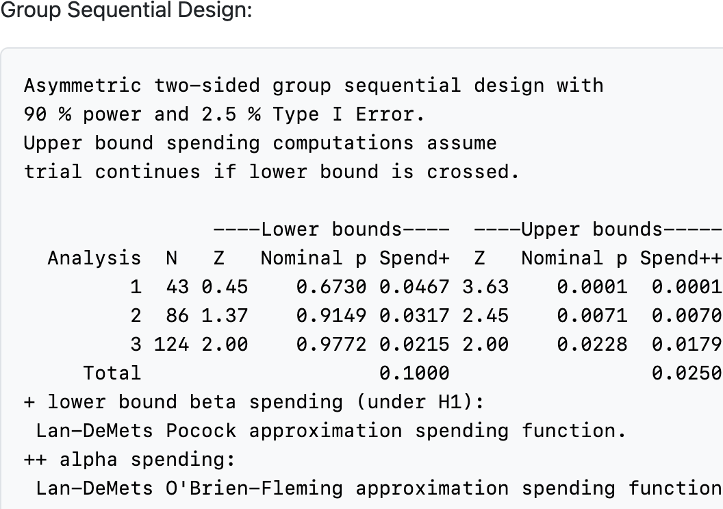
Recall that we have been planning analyses after 35% and 70% of observations are available. For the 35% analysis (t = 0.35), you can see that essentially no \(\alpha\)-spending is planned (solid line), while for the 70% analysis, approximately 30% of the final spending is planned. A much larger proportion of \(\beta\)-spending is planned early in the trial. You can see the actual spending at analyses in the “Text” tab as shown in Figure 8.2.
The \(\alpha\)-spend at each analysis, \(f(t_i) - f (t_{i-1})\), is in the “Spend++” column. The \(\beta\)-spend at each analysis, \(g(t_i) - g(t_{i-1})\), is in the “Spend+” column. You can see that the total \(\alpha\)-spend is equal to the total Type I error of 0.025 and that the total \(\beta\)-spend is equal to the total Type II error of 0.10, or one minus the power. The “Spend+” footnote indicates that \(\beta\)-spending, the probability of crossing a futility bound and stopping under the alternate hypothesis \(H_1\), is in this column. The footnote also provides the spending function used. Finally, this footnote will indicate spending under H0 for the boundary choices with H0 spending selected. The “Spend++” footnote indicates that \(\alpha\)-spending is in this column and indicates the spending function used.
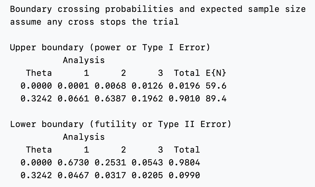
Next, we examine the lower part of the output in the “Text” tab (Figure 8.3). The \(\alpha\)-spending in this table is actually lower than that provided by \(f(t)\) for asymmetric designs with non-binding futility bounds; in this case \(\alpha\)-spending is computed as if crossing the futility bound is ignored. In this table however, probabilities are all computed assuming the trial stops the first time a boundary is crossed. Note that the “Theta” column displays in the lower table is the standardized effect size which is 0 under the null hypothesis and 0.3242 under the alternative hypothesis for this example; further definition of the standardized effect size is beyond the scope of this book; see Jennison and Turnbull (2000). The top row in the “Upper boundary” table indicates the Type I error assuming the trial actually stops and cannot subsequently cross an efficacy bound if a futility bound is crossed; the total Type I error indicated here is 0.0196, less than the 0.025 Type I error that assumes the trial does not stop if the lower bound is crossed. Depending on the spending functions used, especially the \(\beta\)-spending function \(g()\), this can be closer to or further from the design Type I error. Power is in the second row of this table; you can see the probability of first crossing an efficacy bound under the alternate hypothesis at each analysis as well as the total power of 0.90. The lower table shows probabilities of crossing the lower bounds under the null (first row) and alternate (second row) hypotheses.
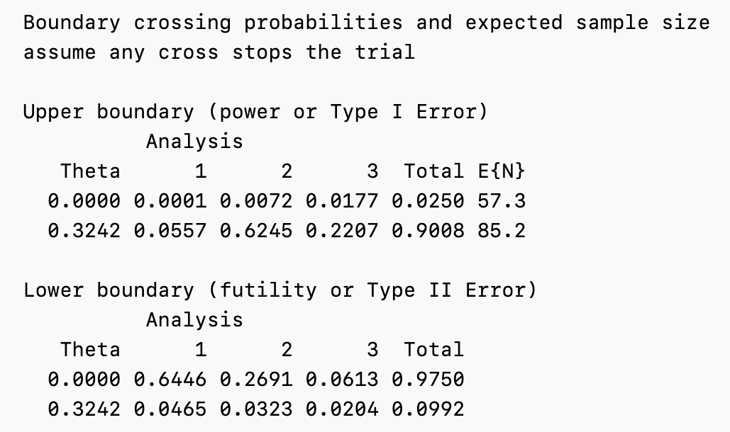
By switching the boundary type to “Asymmetric, binding” in the “Boundaries” input tab, we get \(\alpha\)-spending in the lower table equal to that in the upper table since the spending computations assume crossing any boundary stops the trial and no subsequent bound can be crossed (Figure 8.4).
8.2 Parameter-free spending functions
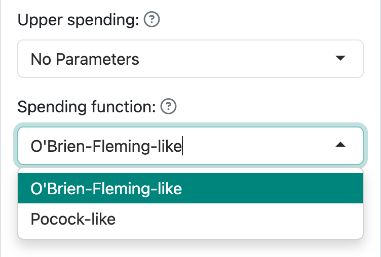
Lan and DeMets (1983) were the first to propose spending functions to control Type I error in group sequential trials. Their methods allowed more flexibility in setting the timing of analyses than previous design methods using boundary families. As specific examples, they proposed spending functions to approximate bounds created using boundary families that were published by Pocock (1977) and O’Brien and Fleming (1979). These spending functions are selected under the “Boundaries” tab using the “No parameters” option as seen in Figure 8.5. The two options under “Spending function” in this case are “O’Brien-Fleming-like” and “Pocock-like.”
8.2.1 Pocock-like bounds
Pocock (1977) efficacy bounds provide equal \(Z\)-values at each efficacy analysis. The “Pocock-like” spending function of Lan and DeMets (1983) approximates this bound as follows for the following design that is otherwise like that in Chapter 2 where a fixed design sample size of 100 was required and the treatment effect that the trial was powered for was \(\delta = 5\). Pocock-like spending bounds were selected for both efficacy and futility.
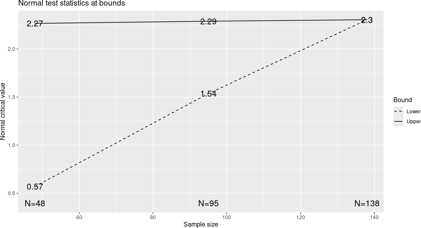
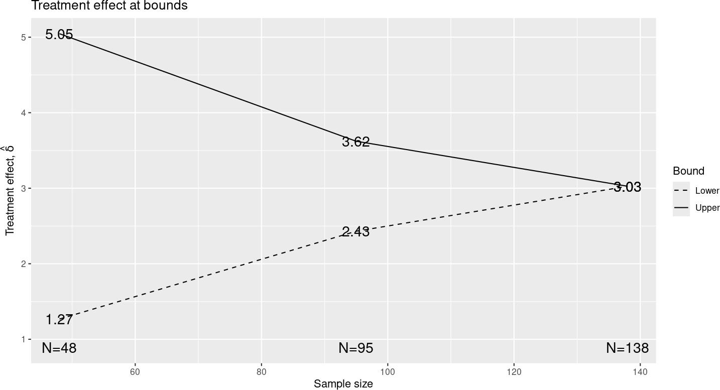
In Figure 8.6, you can see that the upper bounds are approximately equal, but not exactly. Generally, Pocock-like bounds are not used as they increase the maximum sample size substantially over the corresponding fixed design with the same Type I error and power and the treatment effect required to cross an interim efficacy bound can be substantially smaller than that for which the trial is powered. In this case, a treatment effect of \(\hat{\delta} = 3.62\) is estimated to be required to cross the second interim efficacy bound, while the trial was powered to detect a larger treatment effect of \(\delta = 5\). You can see this treatment effect estimate either by selecting the “Treatment effect” plot (Figure 8.7) or by looking under the “Tabular” output tab. Recall that this design is powered to detect \(\delta = 5\). Note that at the second interim we estimate that \(\hat{\delta} = 3.62 < 5\) is required to cross the efficacy bound. Since regulators generally advise against early stopping for efficacy other than for extreme results, this may be a consideration in choosing an even more conservative bound. The treatment effect required to cross the futility bound at the second interim may be undesirably close to what is required at the final analysis to stop the trial.
Pocock-like bounds may be useful in cases such as 1) a trial for a treatment that is already proven for a related condition or 2) an experiment where you just need a statistically significant finding and hope to stop early to establish a proof-of-concept. A Bayesian design with efficacy boundaries similar to a Pocock bound was used for a COVID-19 vaccine trial (Polack et al. 2020), presumably as an effort to accelerate early boundary crossing.
8.2.2 O’Brien-Fleming-like bounds
The O’Brien-Fleming-like spending function is broadly accepted as providing sufficiently stringent interim bounds to stop a trial early. Interim bounds are stricter for O’Brien-Fleming designs than for Pocock designs. They also have the advantage of not substantially increasing the sample size over a fixed design.
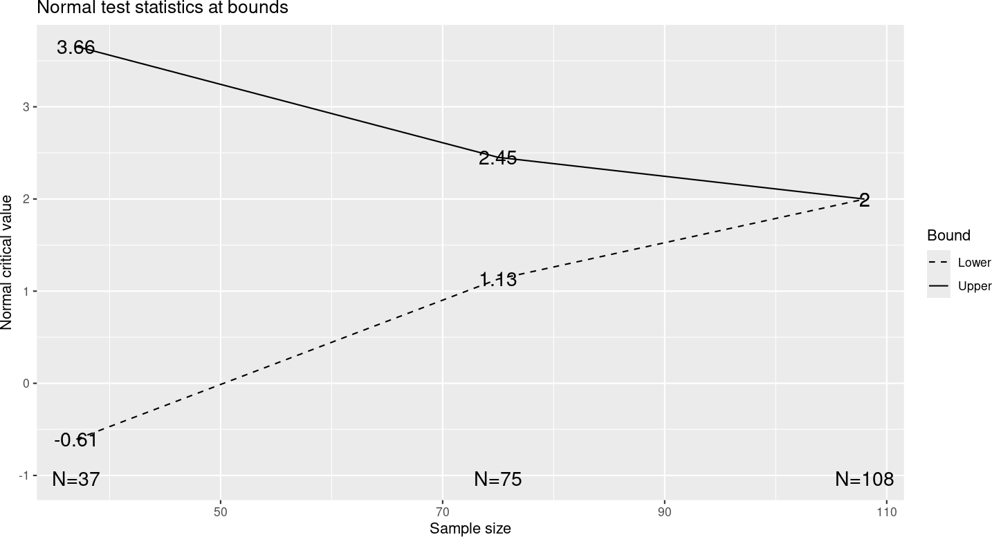
In Figure 8.8, you can see that the \(Z\)-values required to cross the bounds are more extreme for the interim analyses and less extreme for the final analysis than for design with Pocock-like spending functions. The sample size is only increased to 108 from the fixed design requirement of 100 compared to a requirement of 138 using Pocock-like spending functions for both efficacy and futility. Note that if you use an O’Brien-Fleming-like spending function for efficacy and Pocock-like spending function for futility as in the previous section, an intermediate sample size of 124 is required for the group sequential design.
8.3 One-parameter spending functions
We present three families of spending functions here which are defined by a single parameter. Each of these can be used in a similar fashion.
8.3.1 Hwang-Shih-DeCani spending functions
Hwang-Shih-DeCani spending functions are defined with a parameter usually denoted by \(\gamma\); in the web interface, \(\gamma\) can range from \(-20\) to \(10\). Figure 8.9, drawn in R with gsDesign and ggplot2, shows the types of shapes that are included in this family. All the families in this section have a very similar look, with curves ranging from highly convex to highly concave and relative linearity in the middle. You can see that each of the spending function families has curves similar to the Pocock-like and O’Brien-Fleming-like spending function. The Hwang-Shih-DeCani and power spending functions are presumably widely used due to the flexibility they provide.
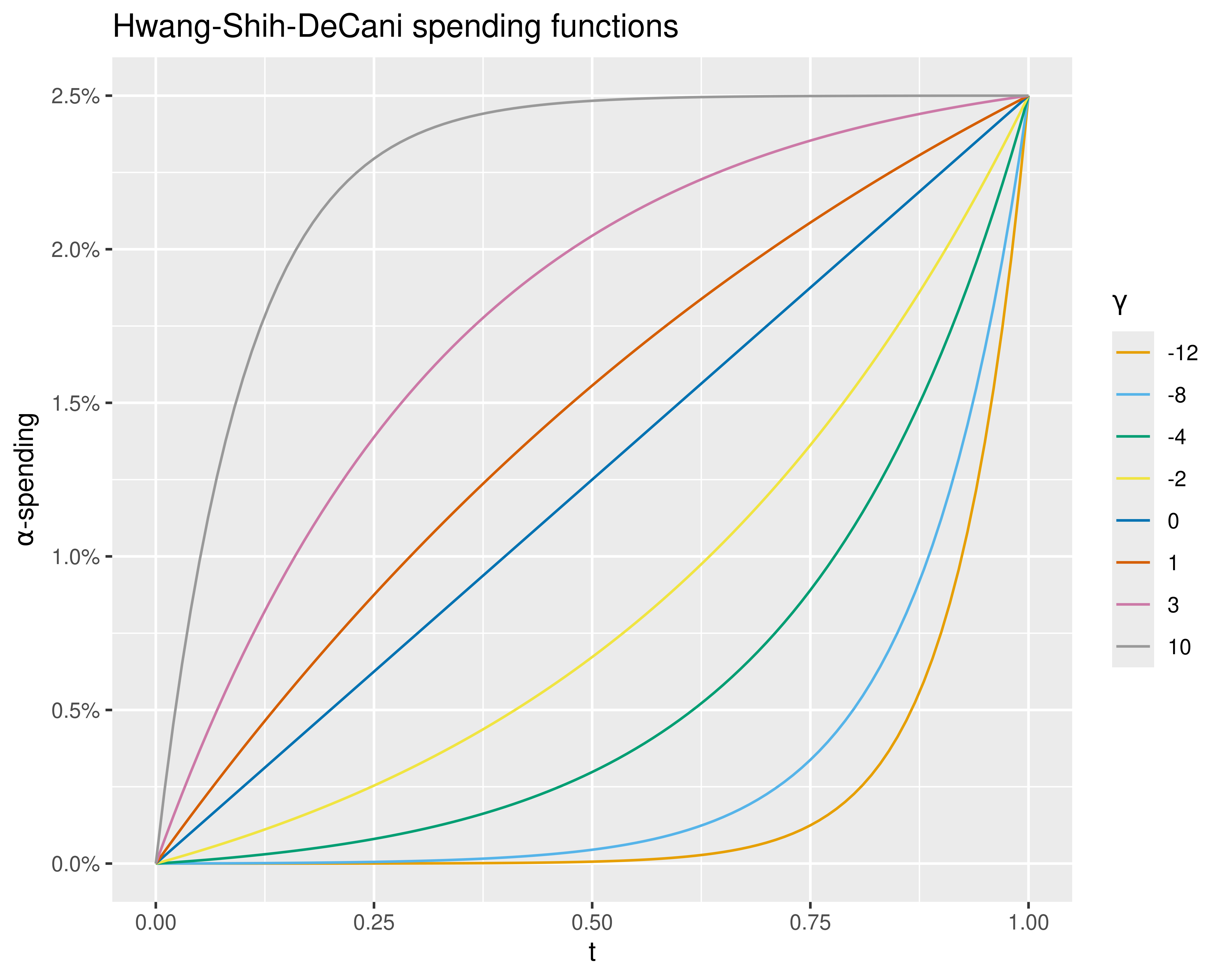
Among the one-parameter families, you can see that the defaults are Hwang-Shih-DeCani spending functions with \(\gamma = -8\) for the efficacy bound and \(\gamma = -2\) for the futility bound. Thus, we will discuss these selections in some detail here. Since the tabular output has all the information we need, we present that in Figure 8.10.
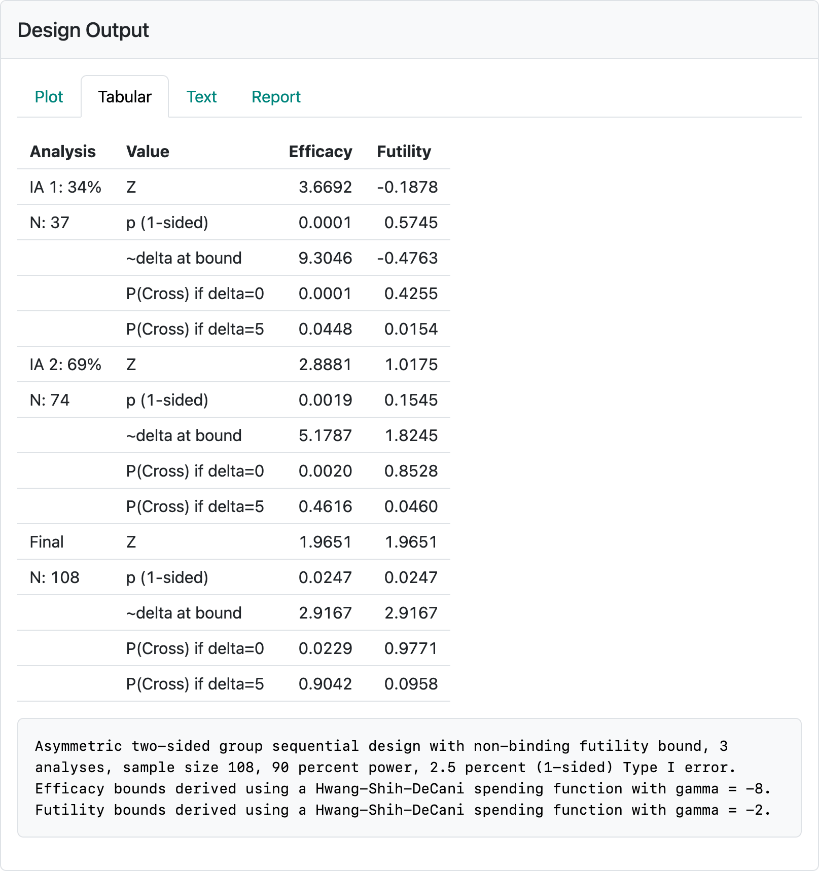
Note that the interim efficacy bounds require very small nominal \(p\)-values for the bounds to be crossed and that the treatment effect (delta at bound) estimated to be needed to cross each bound is bigger than the \(\delta = 0.5\) that we powered the trial for. There is also a minimal increase over the sample size of 100 required for the fixed design. On the other hand, the futility bound at the first interim analysis does not even require a positive trend to continue the trial (\(\hat{\delta} = -0.48\)) and thus might be termed a “disaster” check. This is probably fine for many trials, especially for a treatment that has been previously proven in a related disease condition. The Hwang-Shih-DeCani family is indexed by a parameter normally denoted by \(\gamma\) and has the formula
\[ f(t) = \alpha \frac{1 - \exp (-\gamma t)}{1 - \exp (-\gamma)}. \]
8.3.2 Power spending functions
Power spending functions are commonly presented in Jennison and Turnbull (2000). In Figure 8.11, you can see that the shapes provided are very much like those from the Hwang-Shih-DeCani family.
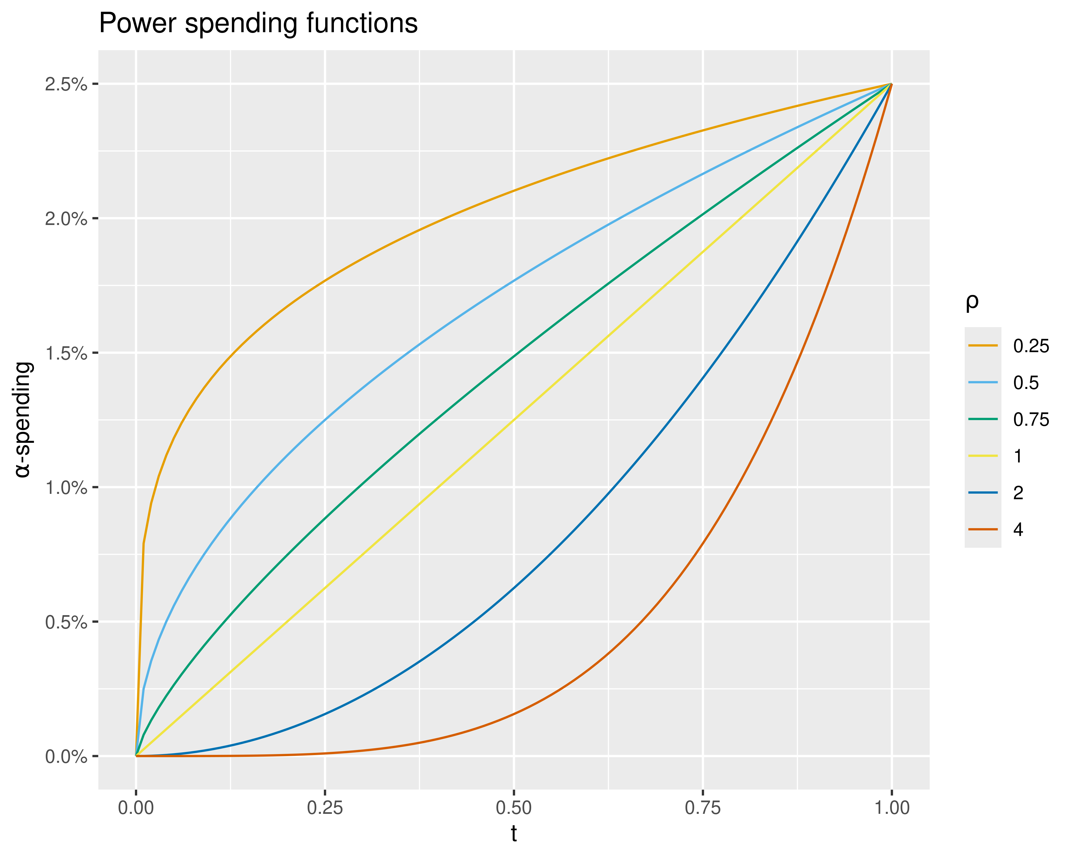
The parameter indexing the power spending function family is denoted by \(\rho > 0\) and the spending function formula is \(f(t) = \alpha \times t^{\rho}\). This formula makes it particularly easy to set the spending value for a single interim analysis. Assume we wish to set \(f(t_1) = x\alpha\) where \(0 < t_1\), \(x < 1\), then we have \(\rho = \log(x) / \log(t_1)\).
8.3.3 Exponential spending functions
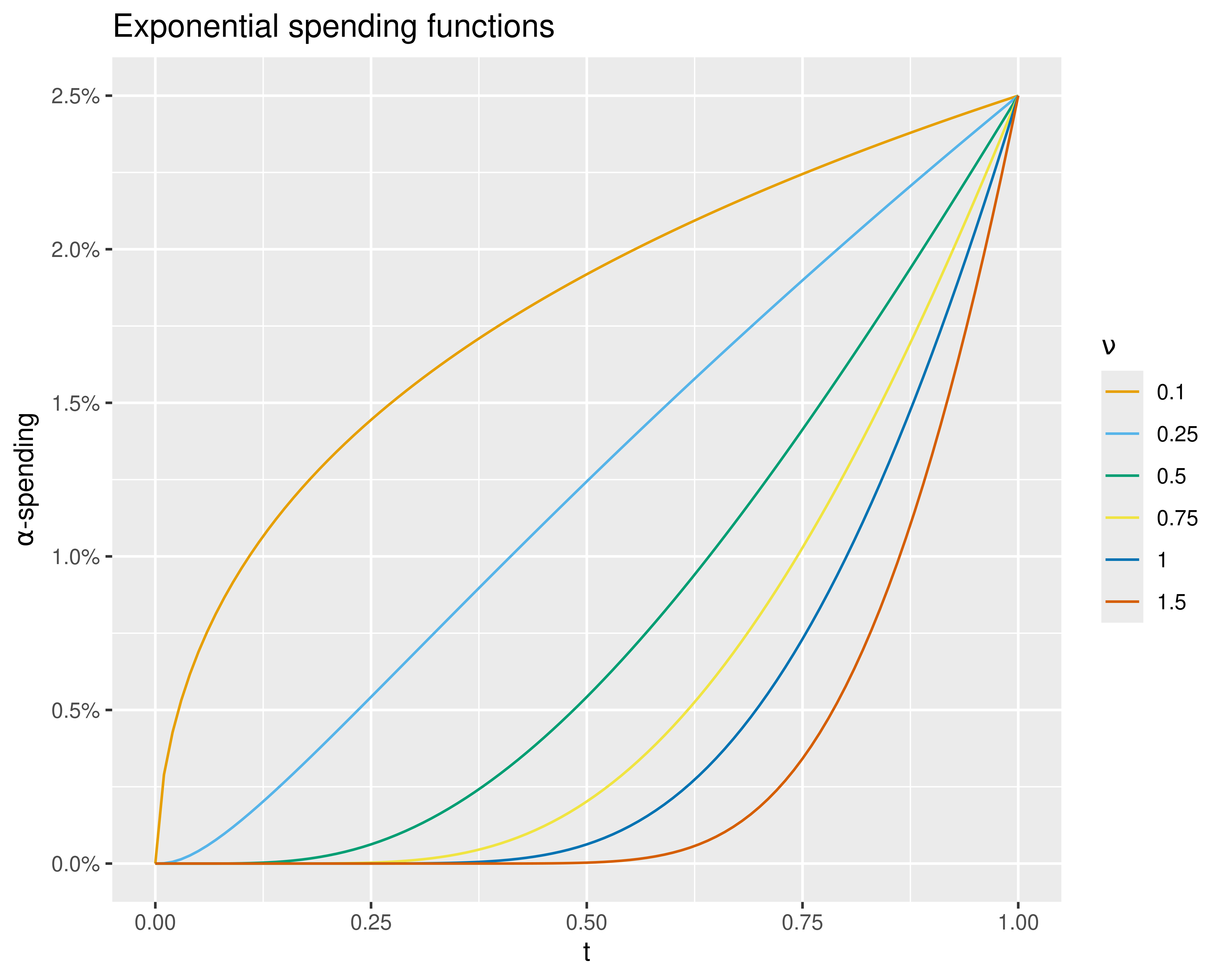
Exponential spending functions take the form \(f(t) = \alpha^{t^{-\nu}}\) where \(0 < \nu \leq 1.5\) in the web interface. As you can see from Figure 8.12, the shapes are like those provided by Hwang-Shih-DeCani and power spending function families.
One thing we have noted is that with \(\nu \approx 0.75\), this can provide a better approximation to actual O’Brien-Fleming bounds than other spending functions. Formally, an O’Brien-Fleming bound takes the form \(c/\sqrt{t_i}\) where \(c\) is a constant depending on \(\alpha\) and the values \(t_i\) representing the fractions of information where analyses are planned. We look at \(B_i = Z_i \times \sqrt{t_i}\) boundaries for \(\nu = 0.75\) for the design we have been using and see that the efficacy bounds are nearly constant, corresponding very closely to constant O’Brien-Fleming bounds (Figure 8.13).
8.4 Piecewise-linear spending functions
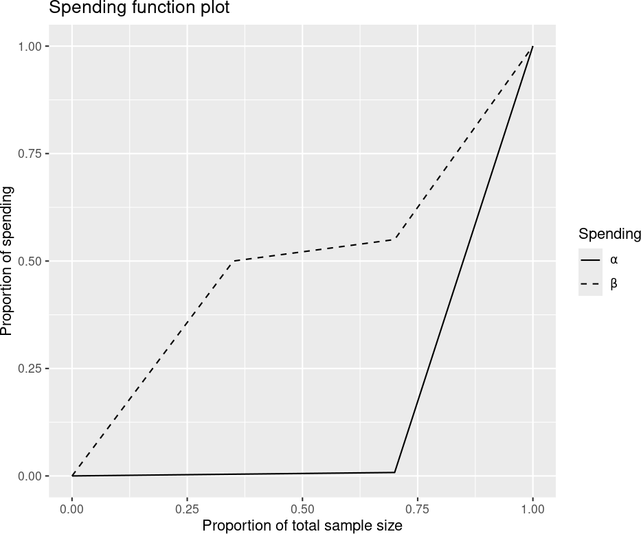
Piecewise-linear spending functions allow you to completely customize the amount of \(\alpha\)-spending and \(\beta\)-spending at each planned analysis as shown in Figure 8.14.
This was produced by setting parameters as Figure 8.15 in the “Boundaries” tab in the input panel.
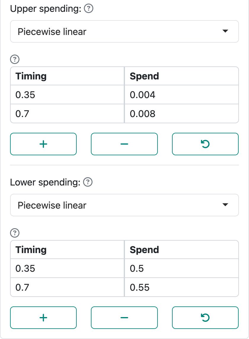
These table inputs allow you to specify values of \(t\), the proportion of sample size at which we wish to define the piecewise-linear spending function, in the left-hand column. In this case, we have used the values of \(t\) where analyses are planned. In the right-hand column, we specify the proportion of the total spending planned the corresponding value of \(t\); i.e., \(f(t) / \alpha\) for \(\alpha\)-spending and \(g(t) / \beta\) for \(\beta\)-spending. We can see that we want to spend half of the Type II error at the first interim and only 5% more at the second interim. The actual spending function values thus require multiplying by \(\alpha\) and \(\beta\), respectively. For \(\alpha\)-spending this means 0.004 \(\times\) 0.025 = 0.0001 at interim 1 and an additional 0.0001 at the second interim.
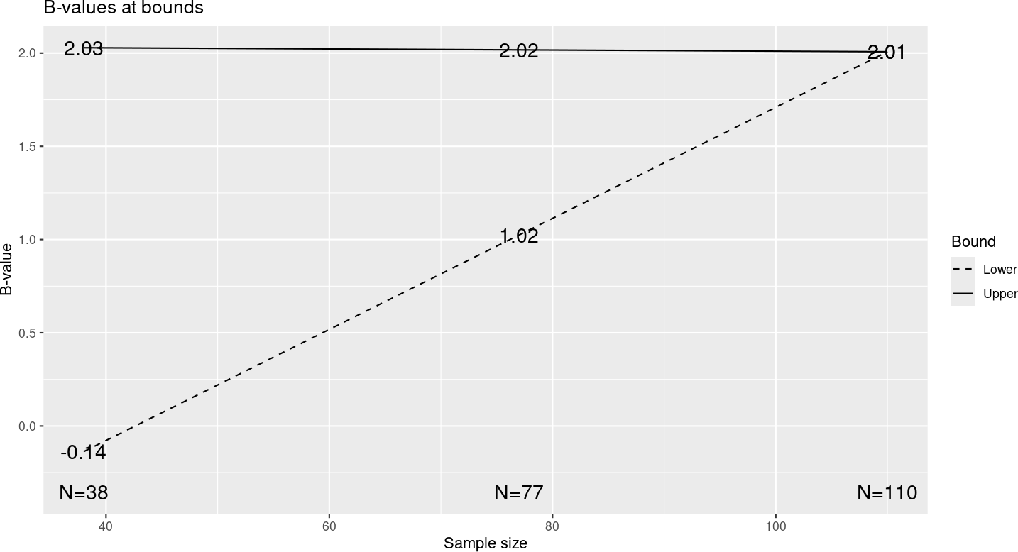
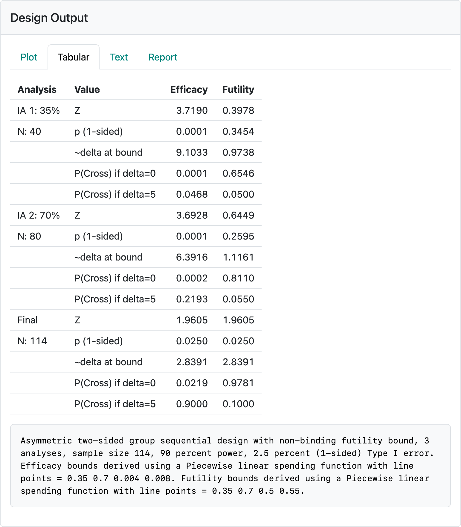
If integer sample size is disabled, these selections result in the summary of the bounds from the “Tabular” output that is shown in Figure 8.16. We note first that the nominal \(p\)-values for efficacy at each interim are 0.0001, which correspond to so-called Haybittle-Peto bounds. The approximate treatment effect required to cross an interim efficacy bound is bigger than the \(\delta = 5\) that the trial is powered for. The futility bound at the first interim gives us a 65% chance of stopping for futility under the null hypothesis (last column, P(Cross if delta=0)). The approximate treatment effect corresponding to crossing this bound is a little less than 1, so at least a positive trend is required to pass the futility analysis. For the second interim where little additional \(\beta\)-spending occurs (little chance to cross the futility bound when the true \(\delta = 5\)), there is still approximately a treatment effect of \(\hat{\delta} = 1\) required to exceed the futility bound. These are the types of evaluations you may wish to consider in selecting bounds.
8.5 2- and 3-parameter spending functions
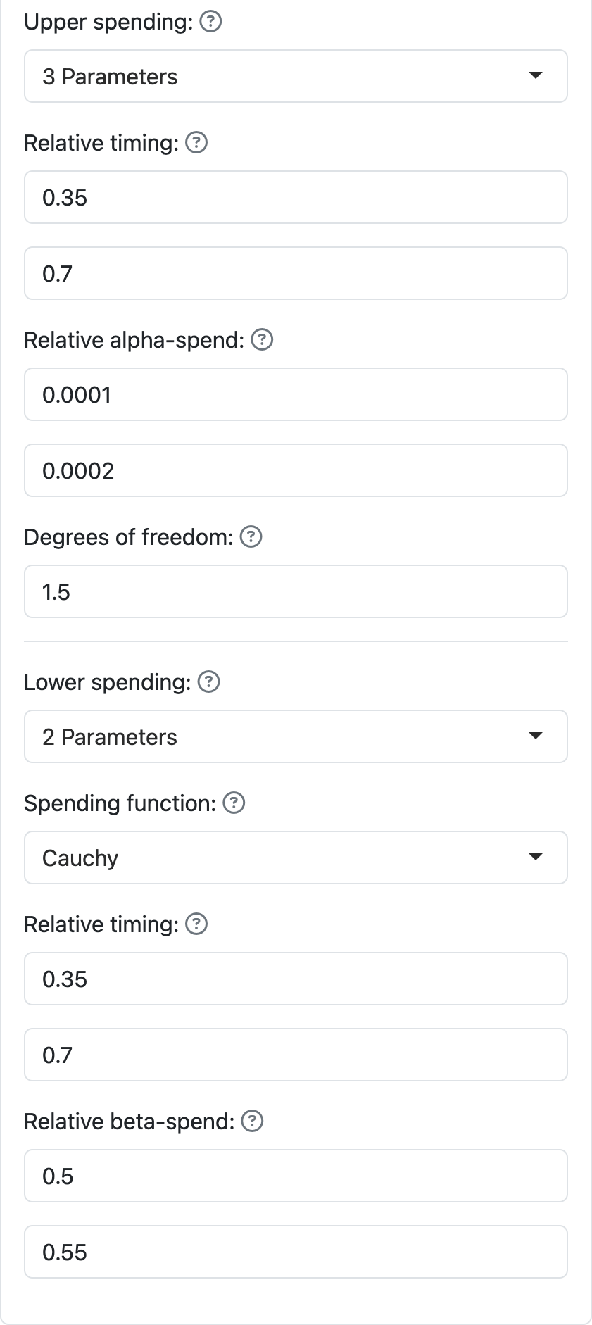
Two- and three-parameter spending functions provide an alternate way for customizing spending at two points in time (Anderson and Clark 2010). The curves are smoother than piecewise-linear, but can only fit spending values at two points with the partial exception of the 3-parameter \(t\)-distribution spending function. The interface looks a little different but is used largely like the piecewise-linear interface as seen in Figure 8.17 where we input relative timing and relative spending for both \(\alpha\)- and \(\beta\)-spending. We have used the same values here as for the piecewise-linear spending functions in the previous section. The \(\beta\)-spending function in this case is the 2-parameter Cauchy spending function, while the \(\alpha\)-spending function is the 3-parameter \(t\)-distribution spending function, in this case with 1.5 degrees of freedom. The rationale for these functions is to provide additional smooth curve options for spending functions beyond the shapes provided by one-parameter spending functions. The smoothing may be preferred when adjusting timing of analyses as in Chapter 9.
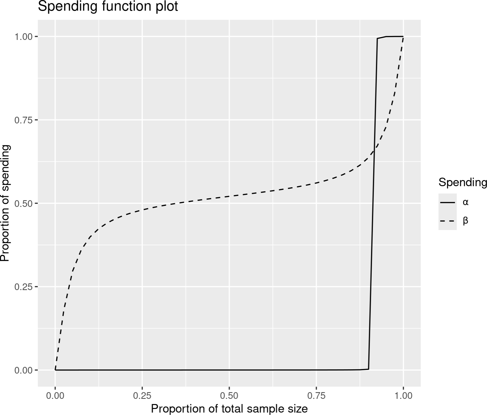
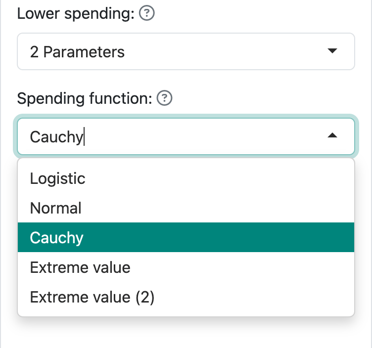
The plot for these two spending functions is shown in Figure 8.18. The Cauchy option was chosen for the \(\beta\)-spending function since it was smoother than the other 2-parameter options shown in Figure 8.19. Note that the \(\alpha\)-spending function implies that any analysis after about 90% of the planned information uses essentially all Type I error that has not previously been spent; if spending is event-based, and you feel you cannot justify the full alpha-spending at the final analysis, this may provide a reasonable alternative. Try the different 2-parameter functions for each spending function as well as the 3-parameter \(t\)-distribution using different values for degrees of freedom. All these functions run through the same values at 0.35 and 0.7 as specified on the previous page. Also try different values for relative spending to see how the spending function curve shapes change.
These spending functions are all of the form
\[f(t) = F(b \times (F^{-1} (t) - a)))\]
where \(a\) is any real number, \(b > 0\) and \(F(t)\) is a cumulative distribution function defined for all real values. Thus, the name of each of these spending function families corresponds to the distribution function \(F(t)\) that is used in the above formula. It is straightforward but beyond the scope of the presentation here to show how to fit these functions through two specified points; see Anderson and Clark (2010).