4 Time-to-event endpoints
Time-to-event endpoints may be the most commonly used endpoints when applying group sequential designs. There is more flexibility allowed in these designs, which means the interface is more complex and there are more examples to go through to explain the variety of options. Thus, this and the next chapter focus on time-to-event endpoints. Chapter 4 focuses more on the interface while Chapter 5 focuses more on example designs.
4.1 Overview and input
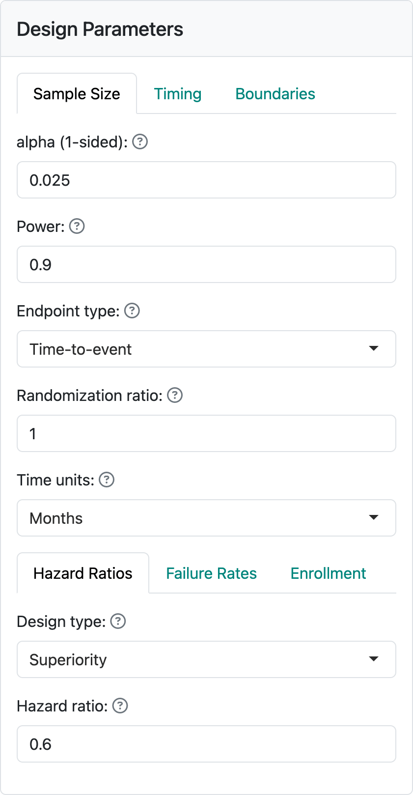
Time-to-event designs in the gsDesign web application and the underlying R package gsDesign currently focus solely on the proportional hazards model. Key factors determining sample size for these designs are the treatment effect under the alternate hypothesis, how fast events are expected to accumulate (failure rates), as well as enrollment rate and duration. As you can see in Figure 4.1, when you select “Time-to-event” as your endpoint type, each of these has its own tab in the input window.
4.1.1 Hazard ratios
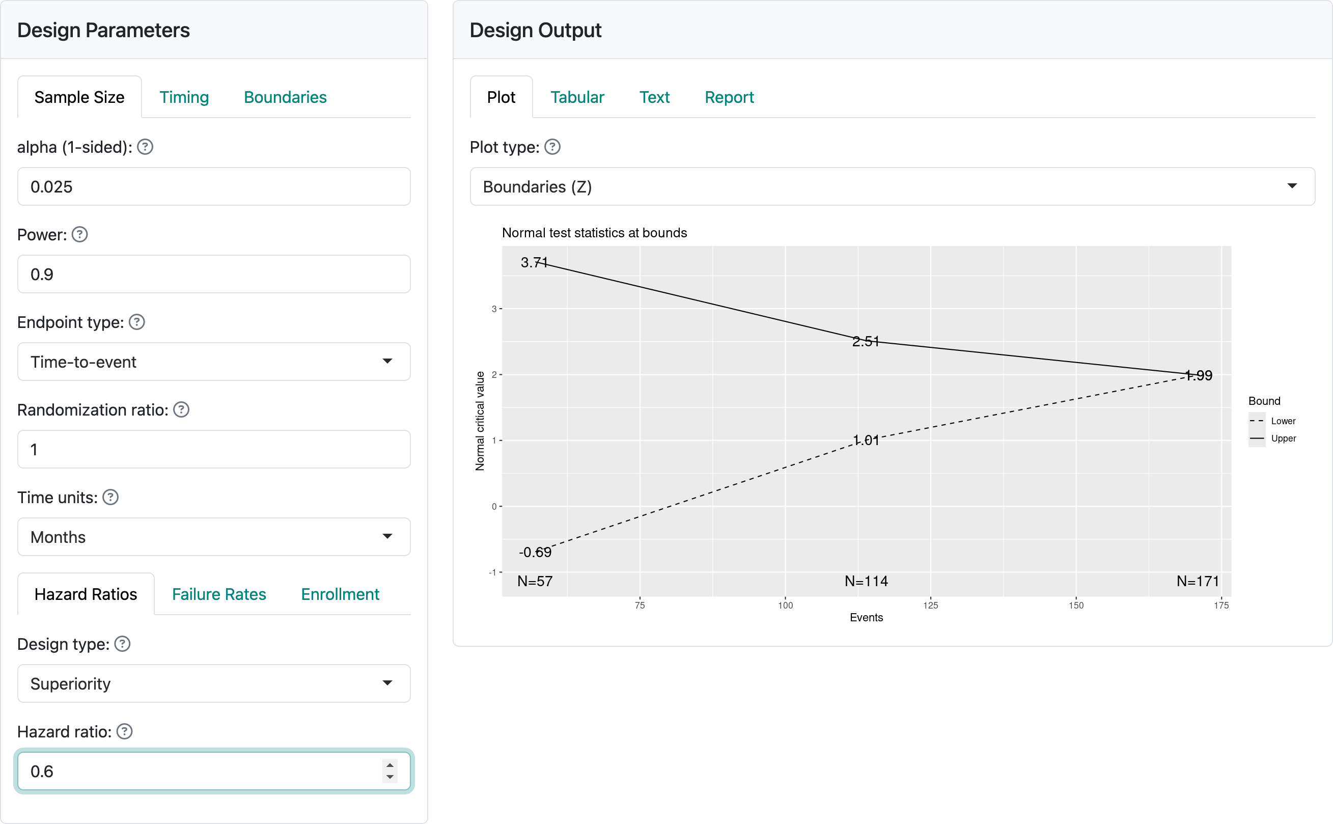
The hazard ratio represents the assumed hazard rate in the experimental group divided by the hazard rate in the control group. Thus, a value less than one indicates a lower hazard for an event in the experimental group, corresponding to a treatment benefit. As previously noted, a constant hazard ratio over time may often not be true, but it is a common assumption both for sample size derivation and for analysis using either the logrank test statistic or the Cox proportional hazards model; we will not describe these here, but they are easily found on the internet or in standard texts. You can see a text box to set the assumed hazard ratio at the bottom of the input screen on the lefthand-side of this page. Here, we have assumed a hazard ratio of 0.6 in Figure 4.2.
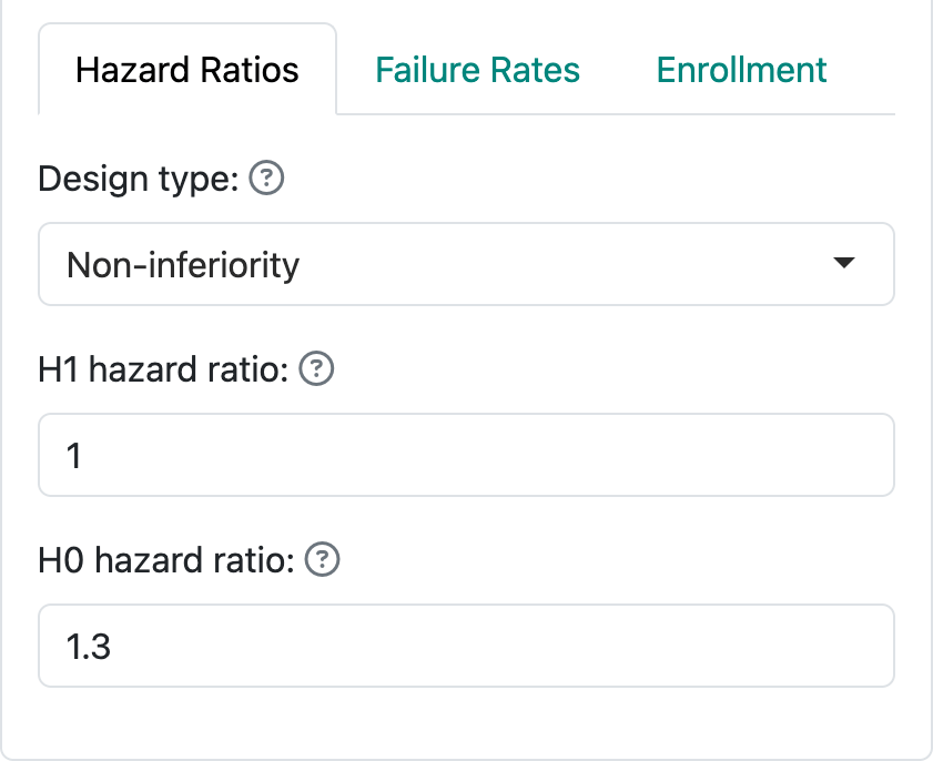
By selecting “Non-inferiority”, you are allowed to set a hazard ratio both for the null and the alternate hypotheses. Most often, the null hypothesis (H0) hazard ratio is set to 1 which means that you are trying to demonstrate superiority of the experimental treatment compared to control. Non-inferiority, or ruling out an H0 hazard ratio greater than 1, may be acceptable if you only need to demonstrate that the experimental treatment is “close to” as good as control (or better). The alternate hypothesis H1 hazard ratio should be set to a value less than the null hypothesis. As an example, for new diabetes drugs, a 2008 FDA Guidance suggested ruling out a hazard ratio of 1.3 for cardiovascular endpoints. While the guidance is no longer in effect, this is still a useful example for the teaching purpose of this book. Figure 4.3 indicates an assumption of no difference under the alternate hypothesis H1 and a trial powered to rule out a hazard ratio of 1.3 under the null hypothesis H0.
4.1.2 Failure rates
Failure rates specify the level of risk/rate of events over time. The web interface focuses primarily on piecewise constant failure rates, which corresponds to a piecewise exponential distribution for the time until an event. Figure 4.4 shows the “Failure Rates” tab where you can specify the failure rate for the control group. Note at the top of the figure you can specify a time unit for the distribution with “Months”, “Weeks”, and “Years” as built in options; this only impacts text in the output.
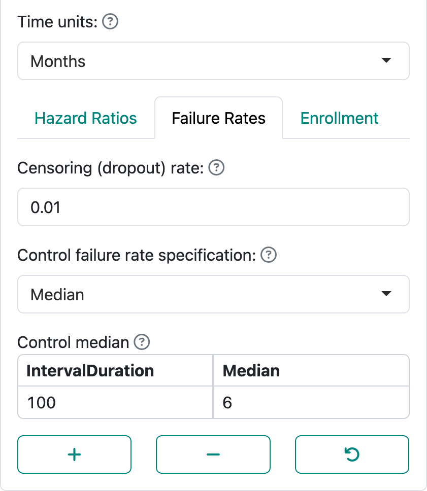
“Control failure rate specification” allows specification of the failure rate using a “Median” or a “Failure rate”. Letting \(\lambda\) denote the failure rate, the probability that the time to event is greater than a value \(t > 0\) is \(P(t) = \exp(-\lambda t)\). A median (\(P(m) = 0.5\)) is simply derived as \(\log(2)/m\). The display in Figure 4.4 demonstrates specification of \(m\). The display in Figure 4.5 demonstrates specification of the failure rate \(\lambda\).
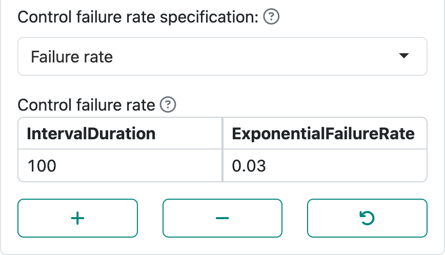
By using the “+” and “-” controls, you can set up intervals with piecewise constant failure rates. For instance, in an oncology trial control treatment may be expected to have a low failure rate initially followed by expectation of a higher rate after disease has had a chance to progress and finally lowering again after high-risk patients have largely failed. Note that the final row in the table is extended to \(\infty\). If you had a study where endpoints only count, say, in the first 6 months, the failure rate after month 6 could be set to 0; this option will be demonstrated in the next chapter.
The combination of the control failure rate plus the hazard ratio specifies the failure rate for the experimental group under the alternate hypothesis. With the above \(\lambda\) for the control group and a hazard ratio of \(0.6\), the experimental group hazard rate under the alternate hypothesis would be \(0.03 \times 0.6 = 0.018\). Starting with a control median \(m = 6\) months and hazard ratio of \(0.6\), the experimental group median is \(6 / 0.6 = 10\) months.
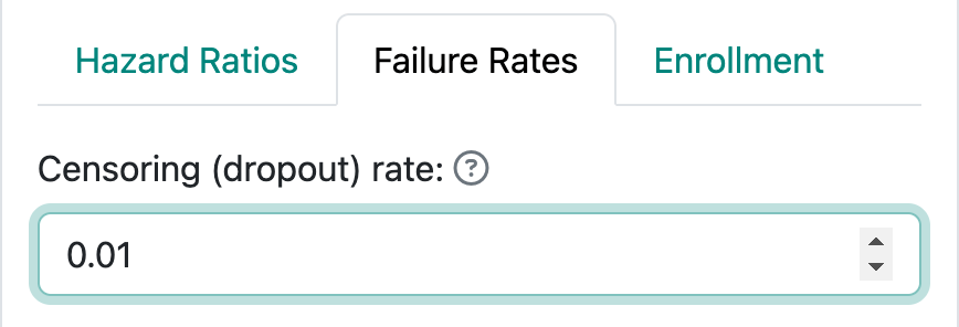
The “Failure Rates” tab also allows specification of censoring or dropout rates. This is always done by specifying an exponential dropout rate that is assumed to be common between the control and experimental groups; when using the R package gsDesign without the web interface, different dropout rates in each group are allowed. Figure 4.6 shows an assumed rate of 0.01 or 1% per month.
Note that the total censoring rate at the end of the trial includes both those who drop out and those who are followed until the final data cutoff for the trial. One simple calculation to explain this follows. We consider a control group with monthly exponential failure rate of 0.01 and monthly exponential dropout rate of 0.005. Time to dropout and time to event are assumed to be independent in commonly-used time-to-event sample size methods, including in gsDesign. Thus, a participant potentially followed for 12 months has the probability of not having an event or being censored equal to:
\[\exp(-12\times 0.01)\exp(-12\times 0.005)=\exp(-12\times 0.015) = 0.835.\] Thus, the total probability of being censored or having an event is \(1 - 0.835 = 0.165.\) Among those having an event or being censored, the proportion with an event is
\[\frac{0.01}{0.01 + 0.005}= 2/3 = 0.110.\] The probability of being censored by 1 year is
\[ (1-\exp(-12\times 0.015))\times 1/3 = 0.055\] Note further that if you want, say, a 5% annual dropout rate we can translate that to a monthly exponential dropout rate \(\eta\) as follows:
\[1 - \exp(-12 \times \eta) = 0.05 \Rightarrow \eta = -\log(1 - 0.05)/ 12 = 0.0043.\]
4.1.3 Enrollment
Figure 4.7 shows the three ways of specifying enrollment assumptions, two of which are recommended over the third.
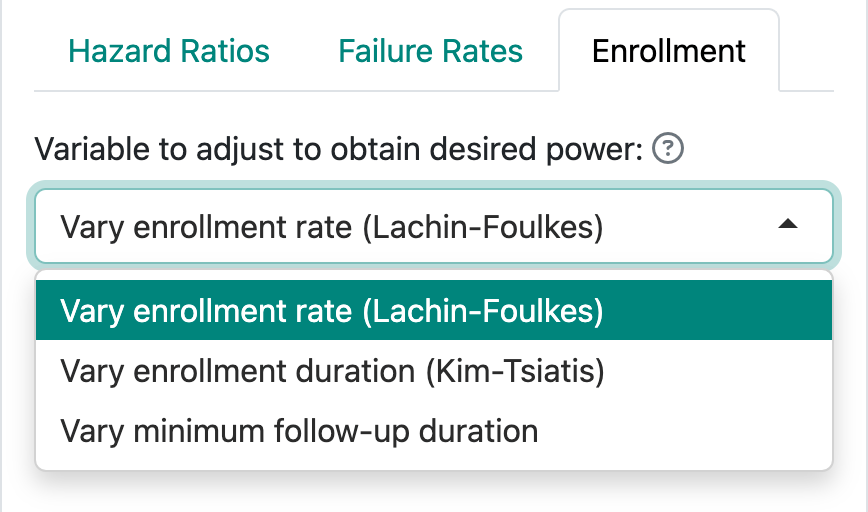
- You can fix the enrollment and follow-up duration and allow the enrollment rate to be computed by gsDesign; this is the Lachin and Foulkes (1986) method. The underlying calculations for fixed design sample sizes are based on this method.
- You can fix the enrollment rate and follow-up duration and allow the enrollment duration to vary. This corresponds to methods suggested by Kim and Tsiatis (1990).
- Finally, you can fix the enrollment duration and rate and allow the follow-up duration to vary to obtain the desired power. This method often creates situations that cannot properly power a trial without adjustment of the enrollment duration or rate.
This chapter focuses on the user interface, while the next chapter focuses on examples.
4.1.3.1 Lachin-Foulkes enrollment assumptions
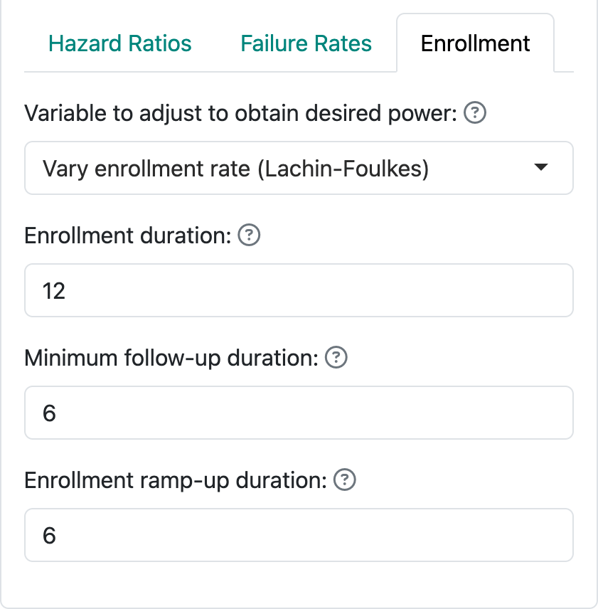
The default enrollment screen is shown in Figure 4.8. This corresponds to the Lachin and Foulkes (1986) method (option 1 above). Here we have specified 12 months of enrollment with an additional 6 months of follow-up. This results in an assumed total study duration of 12 + 6 = 18 months. We are also allowed to specify an “Enrollment ramp-up duration”, which has been set to the first 6 months of enrollment in this case. The enrollment ramp-up period is divided into 3 equally long intervals, 2 months each in this case, during which enrollment rates are assumed to be 25%, 50%, and 75% of the final enrollment rate. This is a simplification of what is allowed when coding in R, but allows substantial flexibility while simplifying the user interface.
When the actual sample size is computed using the Lachin-Foulkes method, the specified relative enrollment rates are fixed and the absolute rates are increased or decreased as needed to obtain the specified power.
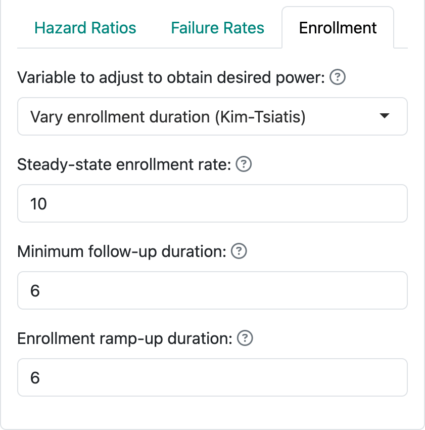
4.1.3.2 Kim-Tsiatis enrollment assumptions
In option 2, we follow methods of Kim and Tsiatis (1990) by fixing the enrollment rates and minimum duration of follow-up, allowing enrollment duration to vary to increase or decrease power to the desired level. Figure 4.9 demonstrates a steady state enrollment rate of 10 patients per month (or week or year, depending on the time unit you specify). This continues for a duration computed by the software and is followed by a minimum follow-up specified here as 6 months. The enrollment ramp-up duration works as before.
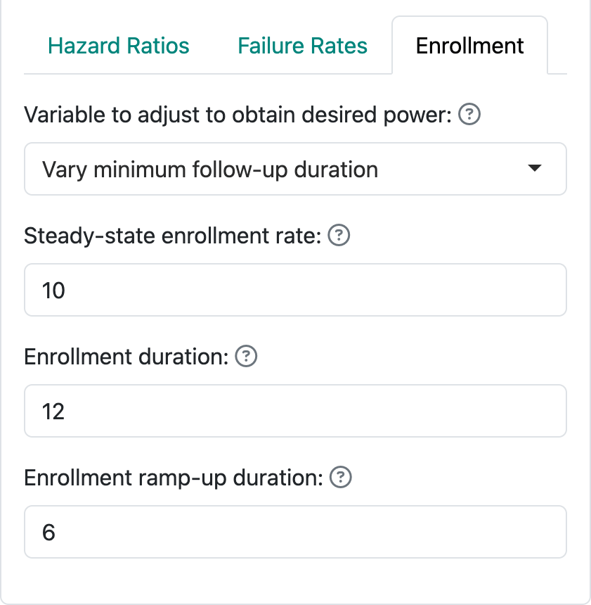
4.1.3.3 Vary minimum follow-up duration
The third, less recommended option for specifying enrollment assumptions is shown in Figure 4.10. In this case, we specify the enrollment rate at steady state (10 per month) and enrollment duration (12 months) and allow the follow-up duration to vary in attempt to achieve the desired power. The enrollment ramp-up duration works as before and is specified as 6 months here. Thus, we here assume an enrollment rate of 2.5 patients per month for 2 months, 5 patients per month for 2 months, 7.5 patients for 2 months, and 10 patients per month for the final six months of the enrollment period. This results in a planned enrollment of \(2 \times (2.5 + 5 + 7.5) + 6 \times 10 = 90\) patients. This helps you realize why this method often fails to produce a solution with the desired power; i.e., more or fewer than 90 patients enrolled over 12 months may be required to produce the desired power and Type I error, regardless of the follow-up duration. With defaults of 90% power, 2.5% one-sided Type I error and a hazard ratio of 0.6, for instance, the rates specified here will not work; changing to a longer enrollment duration (e.g., 24 months) or higher steady state enrollment rate (e.g., 25 per month) result in a solution under these assumptions.
4.1.4 Timing tab
The timing tab allows setting timing not only by information fraction as for all other endpoint types, but also by calendar timing. When you have selected a survival endpoint, the default is to set information fraction as elsewhere and as seen in Figure 4.11.
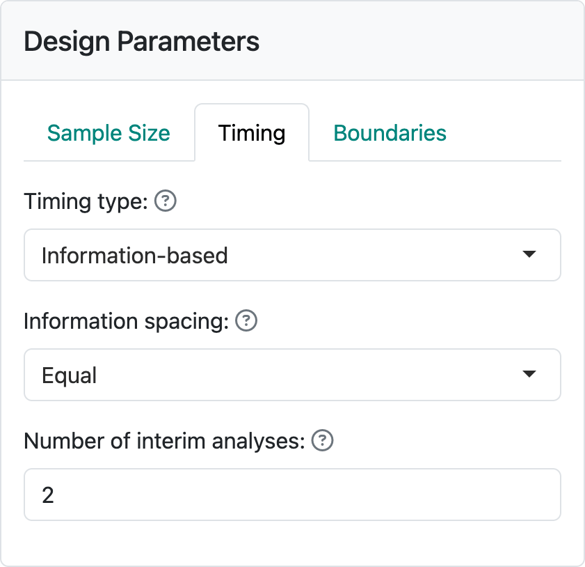
When information-based timing is selected, calendar timing will be computed for you to match the targeted information fractions.
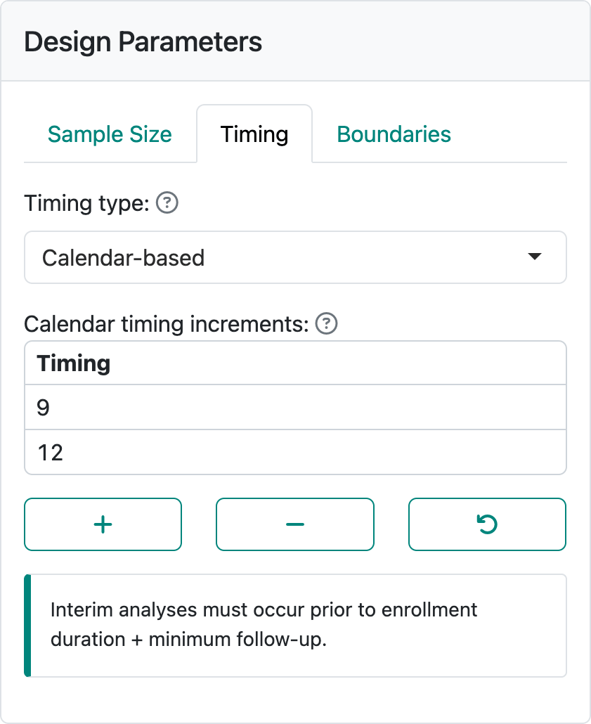
The other alternative is to set timing of analyses by specifying calendar times and computing corresponding information fractions, as shown in Figure 4.12. This option is only available when the Lachin-Foulkes option for enrollment is selected. The interim analyses must be specified before the trial duration which is determined by enrollment duration plus minimum follow-up that you provide in the Enrollment tab.
4.1.5 Example design
Using the above interface components, we select the following options which can be entered or can be loaded from tte-lachin-foulkes.rds.
- Sample Size tab
- Hazard Ratio tab: alpha = 0.025, Power = 0.9, Hazard ratio = 0.7
- Failure Rates tab: Censoring (dropout rate): 0.001, Median = 8
- Enrollment tab
- Enrollment duration: 24
- Minimum follow-up duration: 16
- Enrollment ramp-up duration: 6
- Timing tab
- Interim analyses at information fractions of 0.35, 0.7
- Boundaries tab
- Spending type: Information-based
- Testing: Asymmetric, non-binding
- Upper spending: 1 parameter, Hwang-Shih-DeCani, Gamma = -8
- Lower spending: 1 parameter, Hwang-Shih-DeCani, Gamma = -2
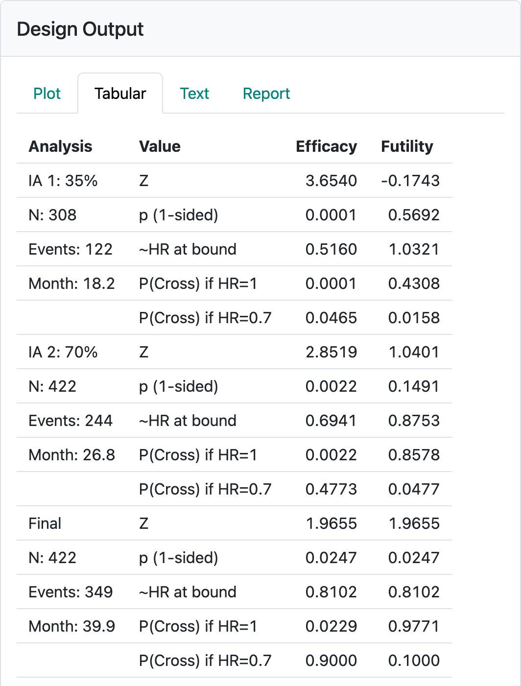
Most of these are as in the previous chapter. The minimum follow-up of 16 was chosen to be twice the median assumed control survival. The resulting design table is modified for time-to-event designs as shown in Figure 4.13.
4.1.6 Boundary update
By selecting Update at the top of the screen, you get the option to enter actual events at the time of each analysis (Figure 4.14).
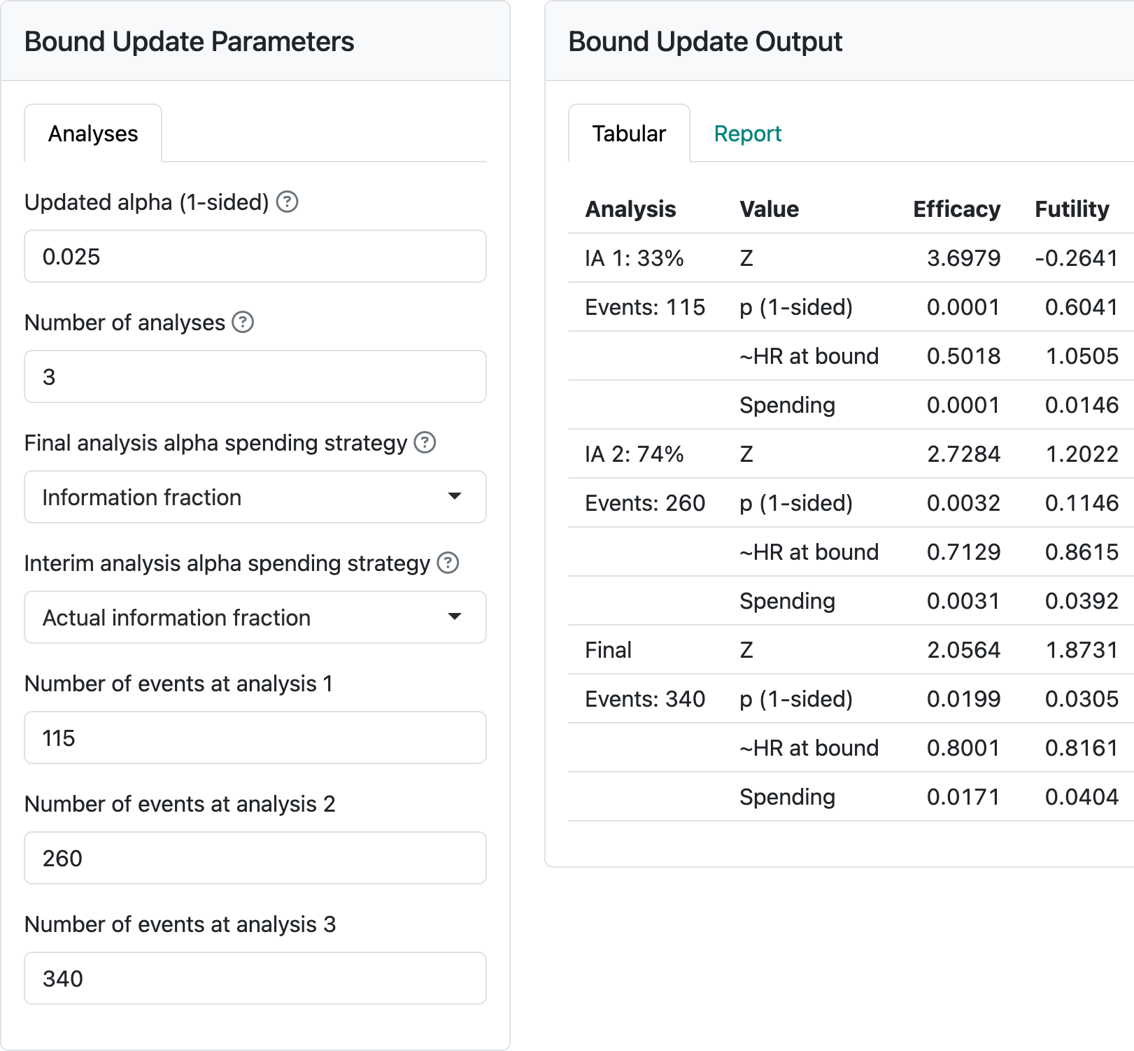
This updates design boundaries. Note the alternatives for spending that are given. The observed (planned) event counts for each analysis are: 115 (122), 260 (244), 340 (349). Normally, information fractions are computed for each analysis based on the actual event counts divided by the final planned event count for the design. Anything other than this should be specified in a protocol. Note in Figure 4.14 that the final targeted event count was not reached at the final analysis. If “Final analysis alpha spending strategy” had been specified as “Information fraction” instead of “Full alpha”, less than the full 2.5% alpha would have been used for the final analysis; the final nominal \(p\)-value would be 0.0199 instead of the 0.0246. Normally, it would be ideal to have the final analysis timing set to achieve the final targeted 349 events from the design. Then there would be no question as to spending the full alpha. Allowing final observed event counts greater than planned does not produce a technical issue for computation of a final nominal \(p\)-value cutoff. For instance, entering 500 for the final event yields a final nominal \(p\)-value cutoff of 0.0237, greater than 0.0199 (due to more alpha spent) and less than 0.0246 (due to smaller correlation between tests) from above. Nonetheless, going substantially over the targeted events is not following the plan while slight deviations can occur due to setting a cutoff date where you estimate the targeted events will accrue. Large deviations may result in being asked to do the analysis when the targeted events accrued, not using the full information available. Finally, we consider adding the “Full alpha” option and under “Interim analysis spending strategy” selecting “Minimum of planned and actual information” yields a final nominal \(p\)-value bound of 0.0248, even larger than 0.246 from above. This is achieved by having a more stringent test at interim 2 where spending is based on the targeted 244 events rather than the observed 260. Again, this strategy should be specified in the protocol if employed.
4.2 Output
4.2.1 Tabular output
We continue the example from the previous section. The tabular output (Figure 4.13) provides a nearly comprehensive summary of a design for a time-to-event study that is easily read and copied into a word processor. Note: the caveat to this copying capability is that you may need to do some table reformatting in your word processor.
The table created here provides information on each interim analysis and the final analysis (Figure 4.13). In the left-hand column, the percent of final required events for the interim analyses and the expected enrollment, number of events and calendar time relative to study start when each analysis is performed is shown.
The right-hand columns show properties of the efficacy and futility bounds:
- \(Z\)-values (normal test statistics) at the bounds.
- Nominal one-sided \(p\)-values at the bounds.
- The approximate hazard ratio at the bounds.
- The probability of crossing a bound under the alternate hypothesis (\(H_1\)).
- The probability of crossing a bound under the null hypothesis.
Using R coding instead of the web interface also allows a summary of conditional or predictive power at the interim bounds. For details, see Section 9.5.
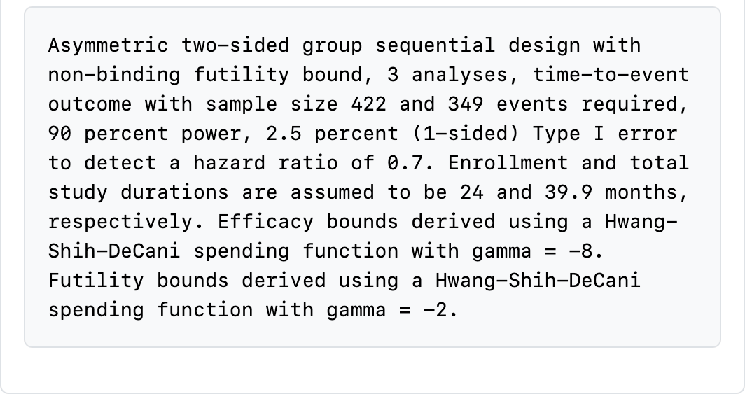
At the bottom of the table, a text string is printed describing many of the design specifications with the exceptions noted above (Figure 4.15). Read through this carefully to see what is there. This will change dynamically as you change input options.
Reading through this table carefully is key to ensuring you have selected a suitable design:
- Aspects of timing include the number of events, enrollment and approximate calendar time for the data cutoff, all in the left-hand column. Questions you might ask include:
- Is the number of events at each analysis suitable, especially at the first interim? In this case, are 122 events sufficient to make any decision? Will you have enough intermediate- to long-term follow-up to feel comfortable with a decision to stop the trial?
- Do the estimated calendar timing and estimated enrollment at each interim analysis make sense? In this case, the first data cutoff is estimated to occur when 308 (73%) of the final targeted 422 have been enrolled even though only 35% of the final number of events are planned for the analysis. Recall that this does not include patients enrolled between the data cutoff and when the evaluation of the analysis takes place. On the “Text” tab (shown shortly), you can see how quickly enrollment is assumed to be proceeding.
- Other questions to ask that can be answered in the righthand-side of the table include:
- Are the approximate hazard ratios at the boundaries acceptable? Would the approximate hazard ratio for a positive trial at an interim be suitable to allow the desired action based on the trial, such as proceeding to the next stage of development or starting a more definitive trial?
- Have you protected the trial suitably from Type I and Type II errors associated with early stopping? Note that “P(Cross) if HR=0” and “P(Cross) if HR=0.7” provide cumulative probabilities of crossing bounds at or before each analysis. Note that because the futility bounds are non-binding, Type I error is still controlled even if the sponsor decides to continue the trial despite crossing a futility bound. It can also be considered optional to stop the trial if an efficacy bound is crossed; this may be done, for instance, if there is insufficient information to fully evaluate the risk-benefit tradeoff or to evaluate one or more secondary efficacy endpoints.
- Are the nominal \(p\)-values in the “p (1-sided)” row likely to be acceptable? These would generally appear in publications.
Note that if you are designing a trial for a new drug or device, you will want to share your design, along with its rationale, with regulators to get their views on the above issues.
4.2.2 Plot output
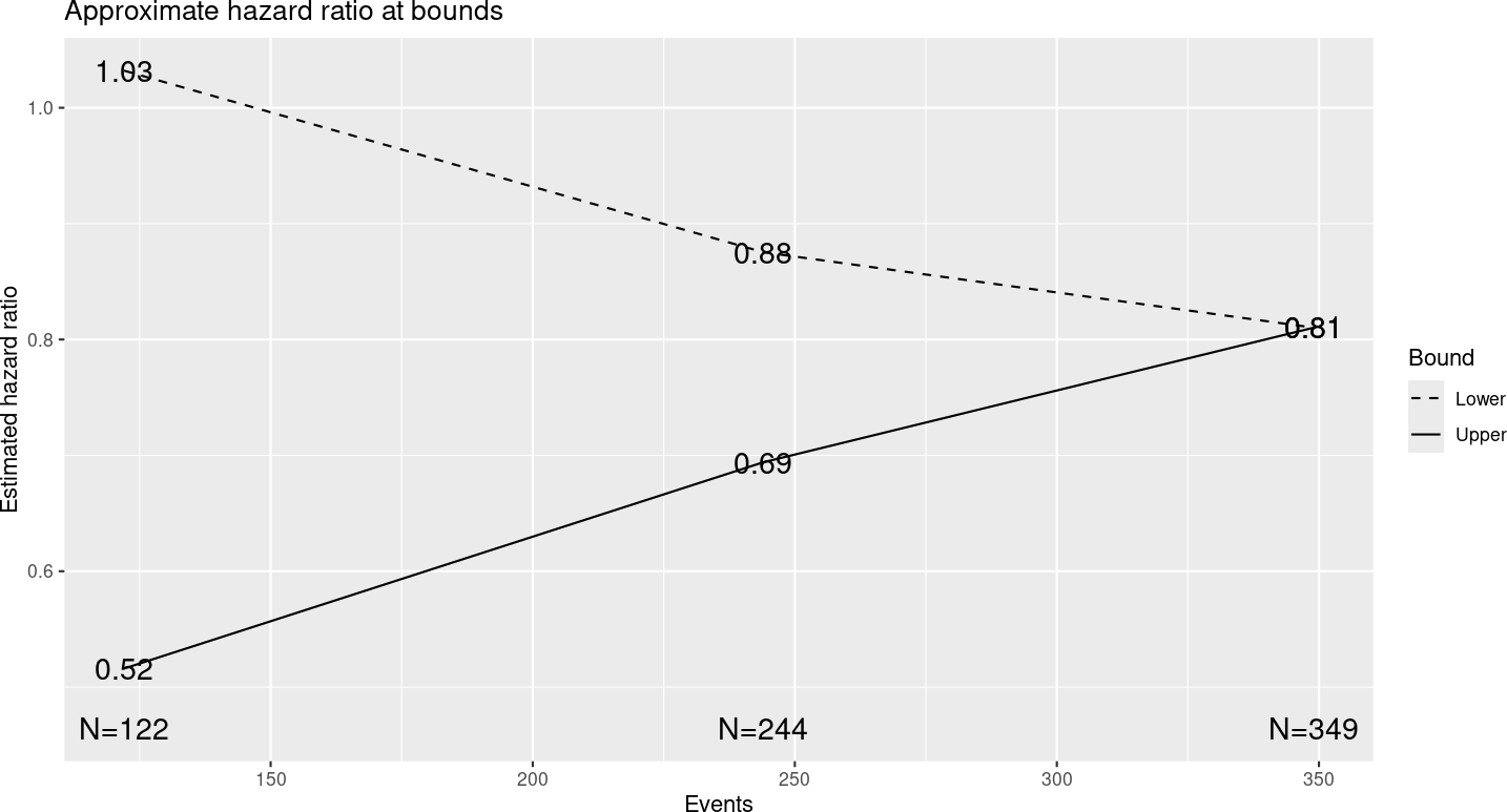
Figure 4.16 shows output from the “Plot” tab demonstrating a plot of the approximate observed hazard ratio required to cross each study bound. Note that you should be able to copy plots from the web browser into a document; resizing the browser window can help to format the plot output as you wish. Exact observed values required to cross any bound may vary somewhat. Note that the x-axis has number of events rather than sample size for time-to-event designs. That is, analyses are generally planned when a pre-specified number of events are available for analysis.
For the specified design, you see that an observed hazard ratio of approximately 1 or greater would be sufficient to cross the lower (futility) bound at the first interim. That is, if the rate of event accumulation in the experimental group is faster (worse), the trial could be stopped for futility at the first interim analysis of 122 endpoint events. On the other hand, a hazard ratio of 0.52 or lower at the first interim, indicating about a 48% lower rate of endpoint accumulation in the experimental group compared to control, would be sufficient to cross the first interim efficacy bound and allow the study to be stopped for efficacy. This plot is important to evaluate whether the properties of bounds are appropriate for your study. In Chapter 8 on spending functions, we will show how the bounds can be changed to match your requirements.
Other plots look very much as before with the exception that sample size is replaced with number of events in all plots displaying sample sizes.
4.2.3 Text output
The following is a direct copy of output for the group sequential design from the “Text” output tab. As you can see, this is fairly lengthy and perhaps less readable than the plot or tabular output. However, it does provide complete information on enrollment rates in addition to what we have seen in other output.
Time to event group sequential design with HR= 0.7
Equal randomization:          ratio=1
Asymmetric two-sided group sequential design with
90 % power and 2.5 % Type I Error.
Upper bound spending computations assume
trial continues if lower bound is crossed.

                 ----Lower bounds----  ----Upper bounds-----
  Analysis  N    Z   Nominal p Spend+  Z   Nominal p Spend++
         1 122 -0.17    0.4308 0.0158 3.65    0.0001  0.0001
         2 244  1.04    0.8509 0.0319 2.85    0.0022  0.0021
         3 349  1.97    0.9753 0.0523 1.97    0.0247  0.0228
     Total                     0.1000                 0.0250
+ lower bound beta spending (under H1):
 Hwang-Shih-DeCani spending function with gamma = -2.
++ alpha spending:
 Hwang-Shih-DeCani spending function with gamma = -8.

Boundary crossing probabilities and expected sample size
assume any cross stops the trial

Upper boundary (power or Type I Error)
          Analysis
   Theta      1      2      3  Total  E{N}
  0.0000 0.0001 0.0021 0.0207 0.0229 206.1
  0.1787 0.0465 0.4308 0.4228 0.9000 286.3

Lower boundary (futility or Type II Error)
          Analysis
   Theta      1      2      3  Total
  0.0000 0.4308 0.4270 0.1192 0.9771
  0.1787 0.0158 0.0319 0.0522 0.1000
             T        n Events HR futility HR efficacy
IA 1  18.24089 306.2693    122       1.032       0.516
IA 2  26.78013 422.0000    244       0.875       0.694
Final 39.88484 422.0000    349       0.810       0.810
Accrual rates:
     Stratum 1
0-2       5.02
2-4      10.05
4-6      15.07
6-24     20.10
Control event rates (H1):
      Stratum 1
0-Inf      0.09
Censoring rates:
      Stratum 1
0-Inf         0
The “Text” tab also is the only place where you can find the sample size required for fixed design without interim analyses (Figure 4.17).
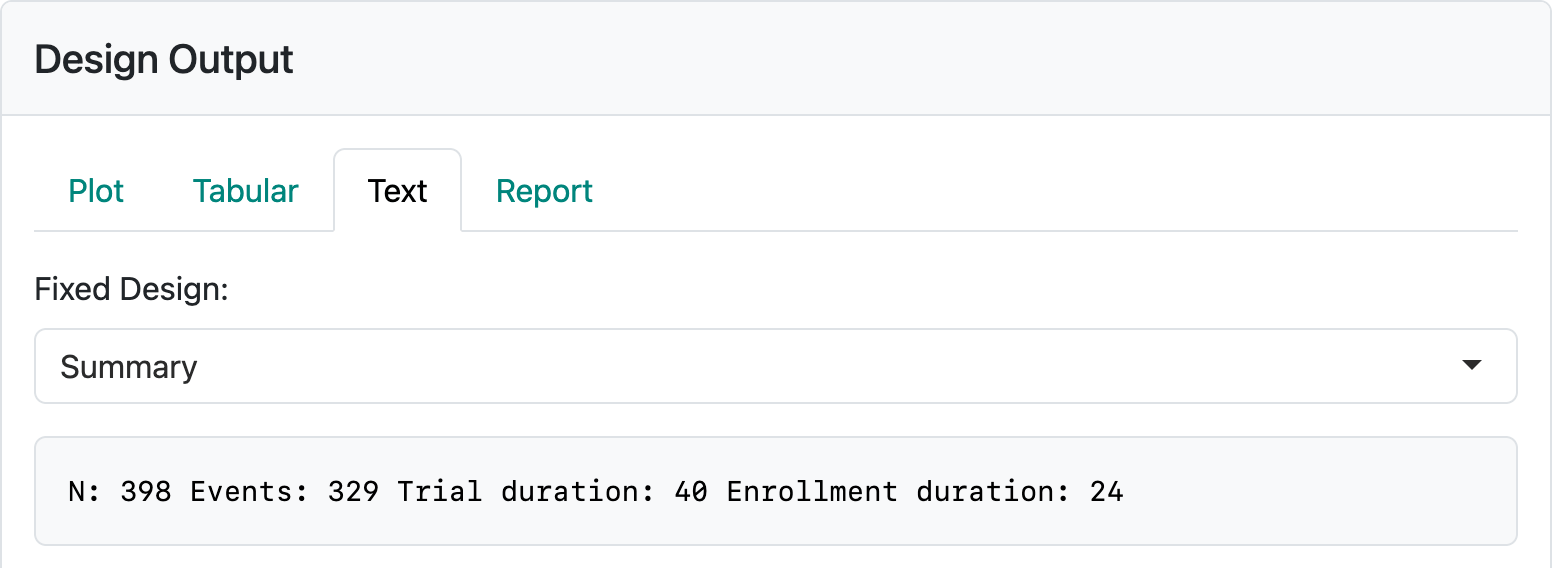
In this case, you can see a sample size of 398 enrolled over 24 months with a 16-month follow-up period resulting in a final analysis at 40 months. There are 329 endpoint events for analysis required at the final analysis. In actually executing the trial, the time to get to the desired enrollment or event count may vary; the final event count of 329 should drive the timing of the analysis.
4.3 Exercises
- Download and open the file from the interface for the above design. Run the report and review the output.
- Play with the “Update” tab to set interim and final analysis options in line with previous sections. Download and run that report.
- Change the Global Options to have continuous sample size and event counts in the above example. Again, download the report and review the code to see how spending is computed.