9 Introduction to R coding

The gsDesign web interface generates code that you may save and reuse in the R programming language. This allows you to reproduce results from the web interface. There are many other capabilities available in R that are not in the web interface. These allow flexibility in the design and analysis of a trial, as well as sample size adaptation.

9.1 Introduction

This chapter covers many topics briefly. We hope the examples presented will be of some use.

The next section begins with notes on how to install R and the gsDesign package used in this book. This section also shows how to access help files and uses a time-to-event trial design as an example. This includes how to update the design when the event counts at analyses differ from planned.

Much of the rest of the chapter is based on an example with normal outcomes. The next two sections show how to derive and then analyze data, including how to update the design when analyses do not have the planned sample sizes or event counts planned. Then we move on to show how to compute conditional and predictive power to predict what the outcome at the end of a trial will be based on interim results. In Section 9.6 and Section 9.7 we show how to update a design based on an interim outcome. First, we show how to update a design based on conditional power followed by demonstrating how to update sample size based on an information-based approach. We finish with information-based sample size adaptation for a trial with a binomial endpoint.

9.2 Some basics

9.2.1 Installing R and gsDesign

In order to use R code to generate the designs in this book, you need to install R and the gsDesign package. R is available at https://cran.r-project.org/. Once R is installed, you should be able to run

install.packages("gsDesign")

which will install not only the gsDesign package, but also other packages that it depends on such as the ggplot2 package.

Although not necessary, you also may wish to install the RStudio IDE (integrated development environment) for R, available at https://posit.co/. The free, open source version of RStudio Desktop can be used by most readers.

9.2.2 Attaching gsDesign

Once you have gone through the above installations, you are ready to run some code generated by the web interface. After you have opened the R console or RStudio IDE, you will need to attach the gsDesign package with the command

library(gsDesign)

This command puts the package in the search path in R, so the functions are directly usable without repeated typing of the namespace. For the rest of the chapter, we assume that you have attached gsDesign in the R session.

9.2.3 Running an initial example

Now go to the “Report” tab in the output panel of the web interface. There you will see 4 blocks of code at the beginning of the file to 1) attach the gsDesign package, 2) enter most parameters for the design, 3) enter failure rates for the design, and 4) derive the design. The latter includes the toInteger() function to adapt the design to an integer-based sample size and integer targeted events at analyses. Following code blocks show how to get a text summary, a tabular bound summary, a plot of design boundaries and a plot of expected enrollment and endpoint accrual.

The note at the bottom of this code will generate which versions of gsDesign and R are run as well as the time the code was generated. Comments (lines starting with the # symbol) tell you what each line of code will do. You will need to run the first line starting with “x <-” in order to derive the design before running the plot, tabular output, or design summary code that summarize the trial exactly as you have seen in the web interface.

Code generated for each endpoint type is different. The supported endpoint types are shown in Figure 9.1.

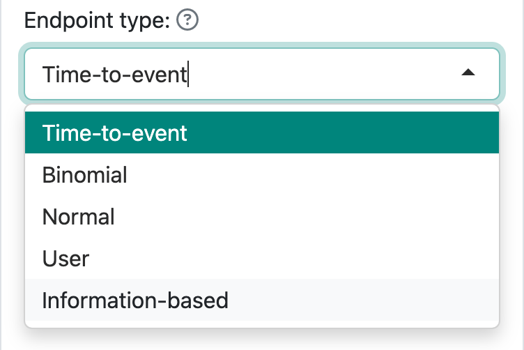
Figure 9.1: Endpoint types supported by the web interface for selection.

All but the “Time-to-event” selection use the gsDesign() function to derive the design. We will demonstrate that along with interim analysis and sample size re-estimation in the following sections.

If you want to know more about the gsDesign(), gsSurv(), nSurv(), nBinomial(), or nNormal() functions from the gsDesign package, help files and vignettes are available with the package and at the documentation website https://keaven.github.io/gsDesign/. Within the RStudio IDE you can get help for gsDesign as seen in Figure 9.2; note that you can scroll down in the interface to see the remainder of the help text. You can also just enter ?gsDesign in the R console window to view the same help text. This chapter is just a brief introduction with examples for some of these and for other functions. The help files should help you understand the functions in more depth. They include function descriptions, input and output specifications, code examples, references, and other details.

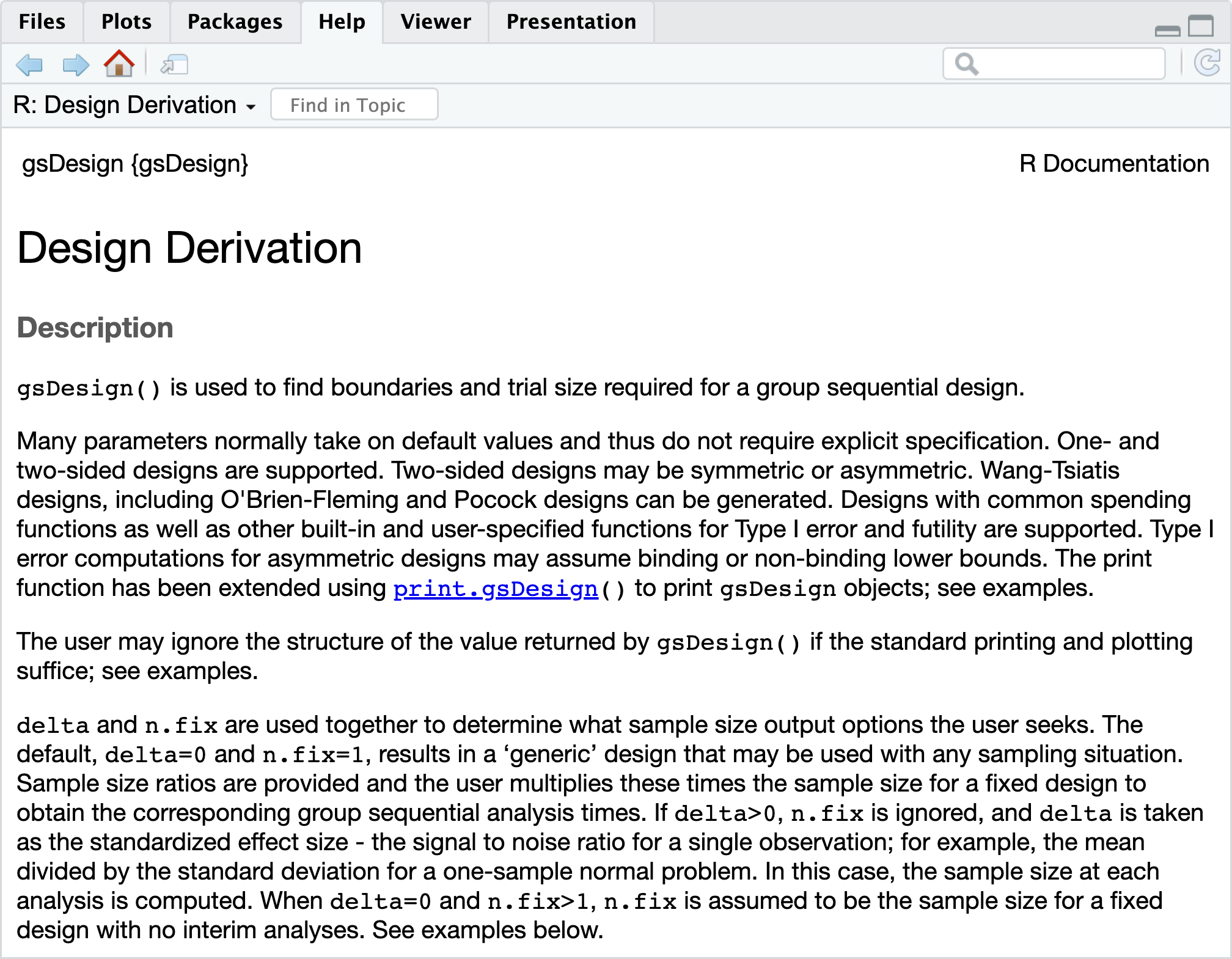
Figure 9.2: Documentation of the `gsDesign()` function displayed in the Help tab of RStudio IDE.

In order to get help on the plot command, you will need to enter ?plot.gsDesign or enter plot.gsDesign in the search field in the Help tab of the RStudio IDE shown in Figure 9.3. The plot.gsDesign() command will plot designs produced by either the gsDesign() or, for time-to-event endpoints, gsSurv() commands. When coding, you can use the shorter plot(x) command as the plot() knows to invoke plot.gsDesign() when x is produced by gsDesign() or gsSurv().

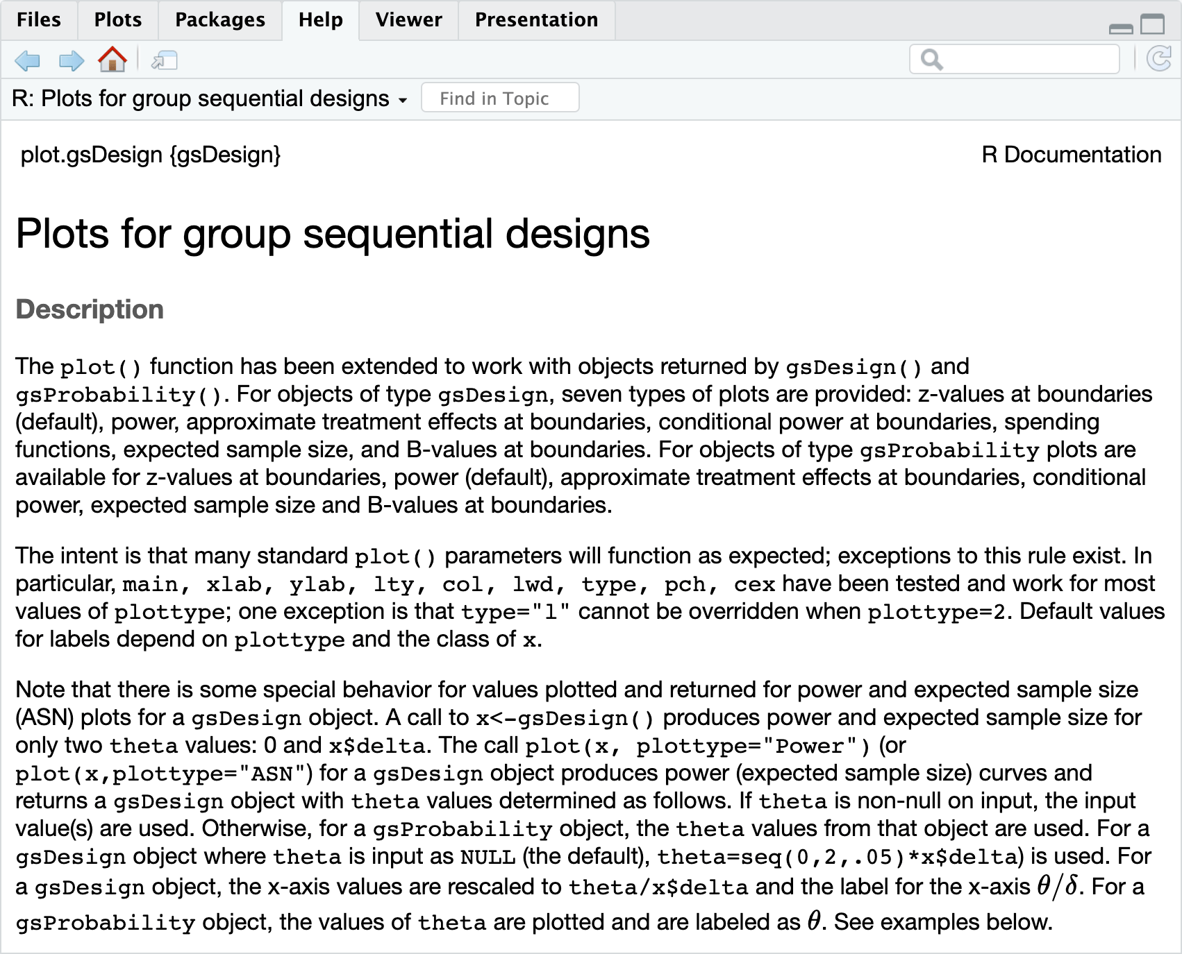
Figure 9.3: Documentation of `plot.gsDesign()` displayed in the Help tab of RStudio IDE.

Finally, to print a summary of the design, you can use gsBoundSummary(x) to print a tabular summary, summary(x) to get a short textual summary, or just enter x and return to get the summary you can see in the “Text” tab of the web interface.

9.2.4 Fixed design sample size and power

To get the fixed design sample size for the normal endpoint trial above, we use the function nNormal().

# Derive normal fixed design
n <- nNormal(
  delta1 = 1,
  delta0 = 0,
  ratio = 1,
  sd = 1,
  sd2 = NULL,
  alpha = 0.025,
  beta = 0.1
)

n
#> [1] 42.02969

We compute the power for this sample size when the standard deviation is larger; note the output includes the power and the input sample size.

# Derive normal fixed design
nNormal(
  n = n,
  delta1 = 1,
  delta0 = 0,
  ratio = 1,
  sd = 1.25,
  sd2 = NULL,
  alpha = 0.025,
  beta = 0.1
)
#> [1] 0.7367143

n
#> [1] 42.02969

For the binomial example powering at 90% with 1-sided Type I error to detect a reduction from a 15% event rate to 10%, we get a fixed sample size with:

nBinomial(
  # Control event rate
  p1 = 0.15,
  # Experimental event rate
  p2 = 0.10,
  # Null hypothesis event rate difference
  # (control - experimental)
  delta0 = 0,
  # 1-sided Type I error
  alpha = 0.025,
  # Type II error (1 - Power)
  beta = 0.1,
  # Experimental/control randomization ratio
  ratio = 1
)
#> [1] 1834.641

If we want more information and more scenarios, we can set the argument outtype = 3 and get a data frame as output. For this example we see the impact a smaller treatment effect on sample size.

nBinomial(
  # Control event rate
  p1 = c(0.15, 0.14),
  # Experimental event rate
  p2 = 0.10,
  # Null hypothesis event rate difference
  # (control - experimental)
  delta0 = 0,
  # 1-sided Type I error
  alpha = 0.025,
  # Type II error (1 - Power)
  beta = 0.1,
  # Experimental/control randomization ratio
  ratio = 1,
  outtype = 3
) |>
  gt::gt() |>
  gt::fmt_number(n_sigfig = 3, columns = 4:14) |>
  gt::fmt_number(decimals = 0, columns = 1:3)

n	n1	n2	alpha	sided	beta	Power	sigma0	sigma1	p1	p2	delta0	p10	p20
1,835	917	917	0.0250	1.00	0.100	0.900	0.661	0.660	0.150	0.100	0	0.125	0.125
2,770	1,385	1,385	0.0250	1.00	0.100	0.900	0.650	0.649	0.140	0.100	0	0.120	0.120

We can also compute power rather than sample size with nBinomial().

nBinomial(
  n = 1500,
  # Control event rate
  p1 = c(0.15, 0.14),
  # Experimental event rate
  p2 = 0.10,
  # Null hypothesis event rate difference
  # (control - experimental)
  delta0 = 0,
  # 1-sided Type I error
  alpha = 0.025,
  # Experimental/control randomization ratio
  ratio = 1,
  outtype = 3
) |>
  gt::gt() |>
  gt::fmt_number(n_sigfig = 3, columns = 4:14) |>
  gt::fmt_number(decimals = 0, columns = 1:3)

n	n1	n2	alpha	sided	beta	Power	sigma0	sigma1	p1	p2	delta0	p10	p20
1,500	750	750	0.0250	1.00	0.166	0.834	0.661	0.660	0.150	0.100	0	0.125	0.125
1,500	750	750	0.0250	1.00	0.336	0.664	0.650	0.649	0.140	0.100	0	0.120	0.120

We can compute power for sample size for a fixed sample size example with nSurv() for a time-to-event endpoint.

# Power is computed when beta is not input
nSurv(
  # Control group failure rate (exponential, median 6)
  lambdaC = log(2) / 6,
  # Underlying hazard ratio (experimental/control)
  hr = 0.5,
  # Dropout rate (exponential, median 40)
  eta = log(2) / 40,
  # Entry rate per time unit (e.g., month)
  gamma = 10,
  # Duration of enrollment
  R = 24,
  # Duration of trial
  T = 36,
  # Minimum follow-up
  minfup = 12,
  # Type II error (`NULL` means it will be computed)
  beta = NULL,
  # 1-sided Type I error
  alpha = 0.025
)
#> Fixed design, two-arm trial with time-to-event
#> outcome (Lachin and Foulkes, 1986).
#> Solving for:  Power 
#> Hazard ratio                  H1/H0=0.5/1
#> Study duration:                   T=36
#> Accrual duration:                   24
#> Min. end-of-study follow-up: minfup=12
#> Expected events (total, H1):        172.9132
#> Expected sample size (total):       240
#> Accrual rates:
#>      Stratum 1
#> 0-24        10
#> Control event rates (H1):
#>       Stratum 1
#> 0-Inf    0.1155
#> Censoring rates:
#>       Stratum 1
#> 0-Inf    0.0173
#> Power:                 100*(1-beta)=99.5431%
#> Type I error (1-sided):   100*alpha=2.5%
#> Equal randomization:          ratio=1

When we use beta = 0.1, the enrollment rate is adjusted to generate the desired 90% power.

# Sample size is computed when beta is input
nSurv(
  lambdaC = log(2) / 6,
  hr = 0.5,
  eta = log(2) / 40,
  gamma = 10, T = 36,
  minfup = 12,
  beta = 0.1
)
#> Fixed design, two-arm trial with time-to-event
#> outcome (Lachin and Foulkes, 1986).
#> Solving for:  Accrual rate 
#> Hazard ratio                  H1/H0=0.5/1
#> Study duration:                   T=36
#> Accrual duration:                   24
#> Min. end-of-study follow-up: minfup=12
#> Expected events (total, H1):        86.3258
#> Expected sample size (total):       119.8184
#> Accrual rates:
#>      Stratum 1
#> 0-24    4.9924
#> Control event rates (H1):
#>       Stratum 1
#> 0-Inf    0.1155
#> Censoring rates:
#>       Stratum 1
#> 0-Inf    0.0173
#> Power:                 100*(1-beta)=90%
#> Type I error (1-sided):   100*alpha=2.5%
#> Equal randomization:          ratio=1

9.3 Design and analysis based on normal outcomes

We demonstrate the basic summary and plotting functions from the gsDesign package for normal outcomes. These can easily be seen for all endpoint types by looking at the report code generated for designs. We assume equal sample sizes in the two groups and compute the total sample size with both arms combined:

n <- nNormal(delta1 = 2, sd = 4, alpha = 0.025, beta = 0.1)
n
#> [1] 168.1188

We would round this up to 170 if actually running a trial with a fixed design. However, for extension to a group sequential design, we convert the unrounded fixed design sample size to a group sequential design with a single interim analysis halfway through. We use many defaults here. See if you can reproduce this design in the web interface; the command summary(x) will give you critical information needed for this.

# Convert to integer sample size
x <- gsDesign(k = 2, n.fix = n, delta1 = 2) |> toInteger()
gsBoundSummary(x)
#>   Analysis               Value Efficacy Futility
#>  IA 1: 50%                   Z   2.7500   0.4167
#>      N: 88         p (1-sided)   0.0030   0.3385
#>                ~delta at bound   2.3452   0.3553
#>            P(Cross) if delta=0   0.0030   0.6615
#>            P(Cross) if delta=2   0.3428   0.0269
#>      Final                   Z   1.9811   1.9811
#>     N: 176         p (1-sided)   0.0238   0.0238
#>                ~delta at bound   1.1947   1.1947
#>            P(Cross) if delta=0   0.0239   0.9761
#>            P(Cross) if delta=2   0.9009   0.0991

Here is the standard textual summary:

summary(x)

#> Asymmetric two-sided group sequential design with
#> non-binding futility bound, 2 analyses, sample size 176, 90
#> percent power, 2.5 percent (1-sided) Type I error. Efficacy
#> bounds derived using a Hwang-Shih-DeCani spending function
#> with gamma = -4. Futility bounds derived using a
#> Hwang-Shih-DeCani spending function with gamma = -2.

In this case, most arguments were set as defaults; if you look at an R Markdown report from the web interface, arguments are spelled out in detail. Once you have reproduced the above design, look at the code tab in the interface when looking at different types of plots to see how you can generate these plots. For instance, to produce a plot of spending functions (Figure 9.4), enter the following code:

plot(
  x,
  plottype = 5,
  xlab = "Proportion of total sample size",
  ylab = "Proportion of spending"
)

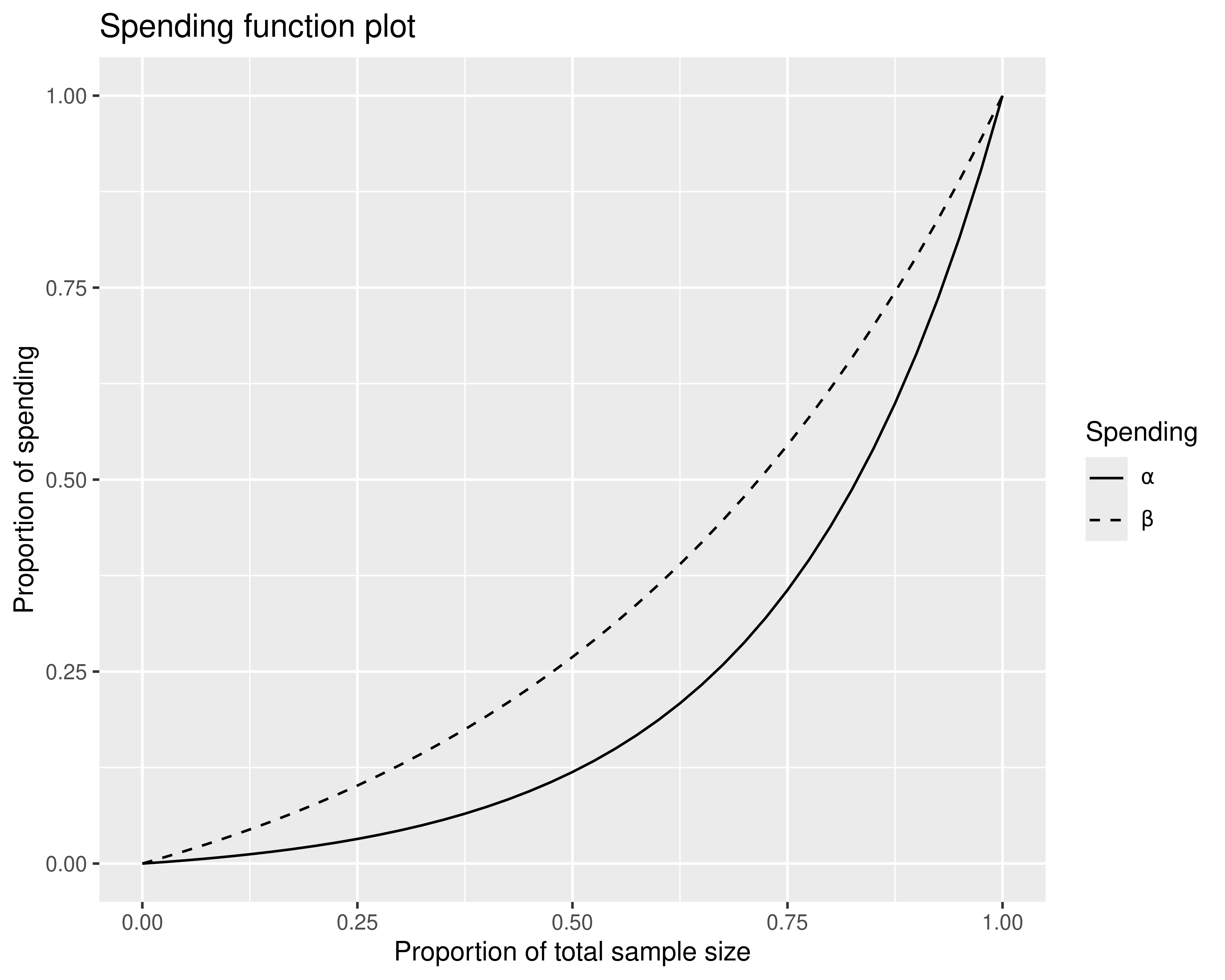
Figure 9.4: Spending function plot using gsDesign.

This code demonstrates how you can change plot types with plottype, as well as how you can change the default labels for the x- and y-axes.

We look at the “standardized effect size” for which the trial is powered and note where this comes from. The variable x$delta contains the standardized effect size. The variable x$theta contains the null treatment effect of 0 as well as the standardized effect size:

x$delta
#> [1] 0.25
x$theta
#> [1] 0.00 0.25

For a normal outcome, the standardized effect size can be derived using the treatment difference and within-group standard deviation. We are looking for a value theta that is a constant times the difference in means for which the trial is powered. The value is such that the estimate of the standardized treatment effect has variance $1/n$ when the total sample size (both arms combined) is $n$.

# Natural parameter: difference in means
delta1 <- 2
# Within group standard deviation
sd <- 4
# Standardized treatment effect
# `2 * sd` is for equal randomization!
delta1 / (2 * sd)
#> [1] 0.25

9.4 Updating a design with normal outcomes

Often analyses do not have exactly the originally-planned sample size or number of events performed. If the numbers are approximately as planned, this should not be an issue. However, the spending function approach taken by the gsDesign package allows you to adjust boundaries to appropriately control Type I error based on the work originally presented by Lan and DeMets (1983).

We assume actual interim analysis is performed after 100 patients instead of the planned 88. We leave the final analysis as planned at 176. To update, we make another call to gsDesign(). Defaults here set Type I and Type II error (alpha, beta), spending functions (sfu, sfl) and corresponding spending function parameters (sfupar, sflpar) to be the same as the original design. If any of these were changed in the call to gsDesign() that provided the original design, the same parameters should be entered here; this is done in detail when you produce an R Markdown report from the web interface. We enter k, the updated design number of analyses, n.fix, the original fixed design sample size, maxn.IPlan, the originally planned maximum sample size for the group sequential design, and n.I, the actual sample sizes at analyses. You can see that the bounds have been updated slightly from the original design. We use the argument exclude = NULL to display all available boundary characteristics available in gsBoundSummary().

xa <- gsDesign(
  k = 2,
  n.fix = n,
  maxn.IPlan = x$n.I[x$k],
  n.I = c(100, 176),
  delta1 = x$delta1
)

gsBoundSummary(xa, exclude = NULL)
#>   Analysis               Value Efficacy Futility
#>  IA 1: 57%                   Z   2.6470   0.6631
#>     N: 100         p (1-sided)   0.0041   0.2536
#>                ~delta at bound   2.1176   0.5305
#>                       Spending   0.0041   0.0331
#>                        B-value   1.9952   0.4998
#>                             CP   0.9899   0.0461
#>                          CP H1   0.9859   0.4673
#>                             PP   0.9592   0.1025
#>            P(Cross) if delta=0   0.0041   0.7464
#>            P(Cross) if delta=2   0.4416   0.0331
#>      Final                   Z   1.9860   1.9826
#>     N: 176         p (1-sided)   0.0235   0.0237
#>                ~delta at bound   1.1976   1.1955
#>                       Spending   0.0209   0.0669
#>                        B-value   1.9860   1.9826
#>            P(Cross) if delta=0   0.0237   0.9761
#>            P(Cross) if delta=2   0.8995   0.1000

We will recreate many of these summaries and discuss them further later in the chapter. For test statistics at bounds, CP (conditional assuming observed treatment effect), CP H1 (conditional power assuming alternate hypothesis treatment effect), and PP (predictive power based on updating a prior distribution for treatment effect) are possibly interesting for interim futility bounds, but otherwise not of great interest. P(Cross) if delta=0 is the cumulative probability under the null hypothesis of crossing a bound at or before a given analysis. In the Efficacy column, this is related to the Spending row which is the incremental probability of crossing an efficacy bound. However, you see the Spending column totals $0.025$ ($0.0041 + 0.0209$) while the cumulative P(Cross) if delta=0 is $0.0237$. This is because for the default of non-binding futility bounds (test.type = 4 in gsDesign()), Spending includes the possibility of crossing the futility bound at the interim analysis and later crossing the efficacy boundary at the final analysis, whereas the $0.0237$ does not count the probability. As noted previously, the Spending represents the preferred way of computing Type I error given that it allows continuation of a trial without inflating Type I error when a futility bound is crossed. All other spending and boundary crossing calculations in the table do not count the probability of crossing one boundary and later crossing another.

The function gsDelta() translates a $Z$-statistic to an approximate treatment effect:

gsDelta(
  # Z-value test statistic
  xa$upper$bound[1],
  # Analysis
  i = 1,
  # Group sequential design
  x = xa
)
#> [1] 2.117585

This matches the value of ~delta at bound (approximate treatment effect required to cross a bound) for the first efficacy bound in the table above. This is based on design assumptions. If translating an observed $Z$-value, this is just an approximation and will differ from the computed observed treatment effect. For time-to-event endpoints, see also gsHR().

9.4.1 Testing, analysis, and repeated confidence interval estimation

Given the above data, we can compute a $Z$-statistic testing the null hypothesis that the difference in means is 0 by dividing the observed mean difference by its estimated standard error. The following example assumes the observed difference in treatment means (natural parameter) at IA 1 is $\hat\delta = 1.4$ and the pooled standard deviation is $5.2$.

# We use updated design
npergroup <- ceiling(xa$n.I[1] / 2)

# Assume pooled standard deviation at IA 1
sdhat1 <- 5.2

# Compute standard error for estimated
# difference in means
sedelta1 <- sqrt(sdhat1^2 * 2 / npergroup)

# Assume observed difference in treatment means
deltahat1 <- 1.4

# Compute interim Z-statistic
z1 <- deltahat1 / sedelta1
z1
#> [1] 1.346154

# Compute standardized treatment effect for observed difference
thetahat <- deltahat1 / (2 * sdhat1)
thetahat
#> [1] 0.1346154

We see that $z1 = 1.35$ is between the futility and efficacy bounds at the interim analysis in spite of having a positive trend.

c(xa$lower$bound[1], xa$upper$bound[1])
#> [1] 0.663069 2.646981

Looking at gsDelta() for the given $Z$-statistic, we see the approximate treatment effect computed under design assumptions is different from the observed treatment effect of 1.2; this is due to the difference in the design and observed standard deviation.

gsDelta(
  # Observed Z-statistic
  z = z1,
  # Analysis
  i = 1,
  # Updated design
  x = xa
)
#> [1] 1.076923

We use the upper $Z$-bound from the updated design to compute a repeated confidence interval for the treatment effect. Repeated confidence intervals are defined as a sequence of intervals for each analysis for which a simultaneous coverage probability is maintained; see Jennison and Turnbull (2000). We see that

deltahat1 + sedelta1 * c(-1, 1) * xa$upper$bound[1]
#> [1] -1.35286  4.15286

These can be done at any planned interim, including planned interims and the final analysis after a boundary has been crossed. You can see that the confidence interval is quite wide at this point, containing both the null hypothesis that the difference in means is 0 and the alternative hypothesis that the difference is 2.

9.5 Conditional power, predictive power, and probability of success

In this section, we cover topics related to predicting what the outcome of a trial will be, either from the start of the trial (probability of success) or at the time of an interim analysis (conditional power, predictive power, conditional probability of success).

9.5.1 Conditional and predictive power

We begin with computing conditional power given an interim result in a trial. We computed the interim normal test statistic $z1 = 1.3461538$ for the trial we designed with normal outcomes. Now we wish to compute the conditional power for the trial at the final analysis given this interim outcome. The functions gsCP() and gsCPz() perform this calculation.

gsCPz(
  # Interim Z-value
  z = z1,
  # Analysis number,
  i = 1,
  # Updated design
  x = xa
)
#> [1] 0.3803728

This value conditions on the observed approximate treatment effect computed using gsDelta() above. If we condition on the H1 treatment effect, we get a higher value:

gsCPz(
  # Interim Z-value
  z = z1,
  # Analysis number,
  i = 1,
  # Standardized treatment effect of design
  theta = xa$delta,
  # Updated design
  x = xa
)
#> [1] 0.7584727

If we condition on no treatment effect, we get the conditional error which could be used to adapt the design (Müller and Schäfer 2004):

gsCPz(
  # Interim Z-value a
  z = z1,
  # Analysis number,
  i = 1,
  # No treatment effect
  theta = 0,
  # Updated design
  x = xa
)
#> [1] 0.069697

We demonstrate a conditional power plot that may be of some use. We will assume a wide range of potential underlying hazard ratios for future events.

delta1 <- seq(-0.5, 4, 0.1)

We compute conditional probabilities based on the observed interim 1 $Z$-value over this range:

cp <- gsCP(
  # Updated design
  x = xa,
  # Analysis
  i = 1,
  # Interim Z-value
  zi = z1,
  # Standardized treatment effects considered
  theta = xa$delta / xa$delta1 * delta1
)

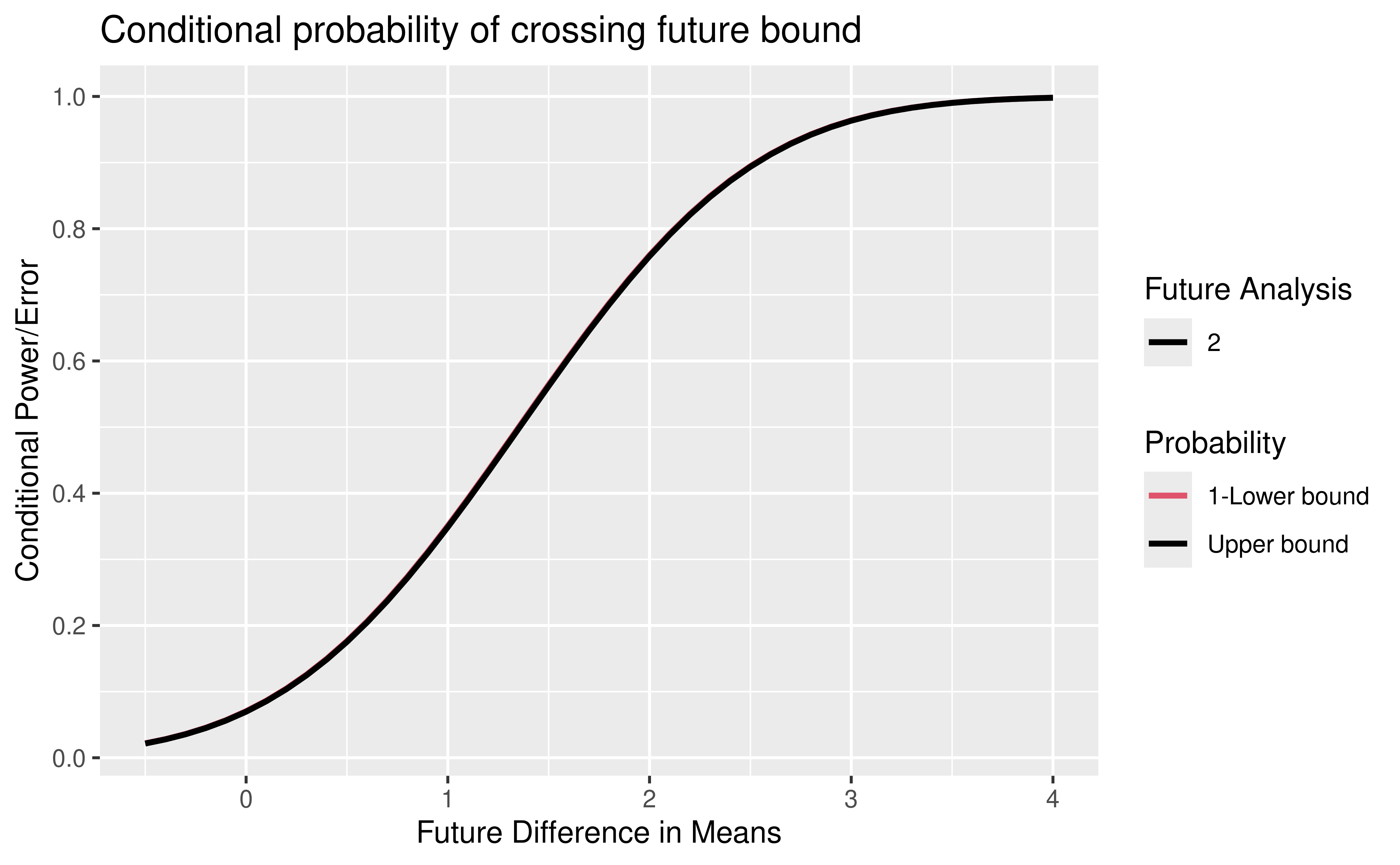
We plot conditional power as a function of future observation underlying difference in means (Figure 9.5). Note the use of the power plot option for the gsDesign plot function. The offset = 1 argument changes the legend to be labeled with “Future Analysis” 2 and 3. The solid black line shows the conditional probability of crossing any future bound prior to crossing a lower bound. More lines would be shown if there were more than one future analysis. In general, black lines on this plot will show the cumulative conditional probability of crossing an efficacy bound prior to crossing a lower bound by the time of any given future analysis by different underlying treatment effect assumptions. The red lines that would be shown if more than one analysis were remaining and would show 1 minus the cumulative conditional probability of crossing a lower bound prior to crossing an efficacy bound by any given future analysis by different underlying treatment effect (HR) assumptions. In order to visualize the red lines, you can see a variation of this in the interface for power at the time of design by selecting the power plot.

plot(
  cp,
  xval = delta1,
  xlab = "Future Difference in Means",
  ylab = "Conditional Power/Error",
  main = "Conditional probability of crossing future bound",
  offset = 1
)

Figure 9.5: Conditional power plot using gsDesign.

The gsCP() function produces another group sequential design, in this case with only one analysis.

gsCP(
  # Updated design
  x = xa,
  # Analysis number
  i = 1,
  # Interim Z-value
  z = z1
)
#>              Lower bounds   Upper bounds
#>   Analysis N   Z   Nominal p  Z   Nominal p
#>          1 76 1.47    0.9296 1.48    0.0697
#> 
#> Boundary crossing probabilities and expected sample size assume
#> any cross stops the trial
#> 
#> Upper boundary
#>           Analysis
#>    Theta      1  Total E{N}
#>   0.1346 0.3804 0.3804   76
#>   0.0000 0.0697 0.0697   76
#>   0.2500 0.7585 0.7585   76
#> 
#> Lower boundary
#>           Analysis
#>    Theta      1  Total
#>   0.1346 0.6177 0.6177
#>   0.0000 0.9296 0.9296
#>   0.2500 0.2399 0.2399

The top table tells us that if we computed a $Z$-statistic only for the post interim analyses and achieved a nominal $p = 0.0697$, we would have a positive result by the method of Müller and Schäfer (2004). Normally, we would just compute based on the combined and use the bound from the updated design.

The relevant table in the above output table produced by the above gsCP() call is the upper boundary table which provides the power of a positive trial given the input interim $Z$-value assuming:

The interim estimated standardized treatment effect theta = 0.1346 with a conditional power of 0.3804.
No treatment effect theta = 0; in this case, the “conditional power” is actually the conditional error or Type I error of a positive result, 0.0697, since there is no treatment effect.
The originally targeted standardized effect size theta = 0.25 with a conditional power of 0.7585. The first of these is what people usually mean by conditional power.

From the repeated confidence interval above, we see that there is a great deal of uncertainty about what the actual treatment effect is at the time of the interim analysis. To account for this uncertainty in predicting the outcome of the trial at the end of the trial, we compute predictive power. This requires assuming a prior distribution for the treatment effect at the beginning of the trial, updating this prior based on the interim treatment result, and averaging the conditional power of a positive finding across this updated prior (i.e., posterior) distribution. The calculation can be done with different prior distributions to evaluate the sensitivity of the result to the prior distribution assumed. Here, we assume a prior distribution for the standardized treatment effect that is “slightly negative” in that we assume the mean of the prior is 0, but the standard deviation for the prior is large so that the predictive power is impacted mainly on the data and not the prior.

prior <- normalGrid(mu = 0, sigma = 3 * x$delta)

Now we proceed to compute the predictive power based on this prior and the interim result. As previously noted, the prior is updated by the interim result in this computation.

# Prior and interim result
pp <- gsPP(
  # Updated design
  x = xa,
  # Observed result
  zi = z1,
  # First interim
  i = 1,
  # Prior standardized effect size values
  theta = prior$z,
  # Weights reflection prior distribution
  wgts = prior$wgts
)

pp
#> [1] 0.4028769

We see that the resulting predictive probability is similar to the conditional power based on the observed outcome (0.4) predictive power vs. 0.38 conditional power. This does not change much if the prior is centered around half the design treatment effect yielding a predictive power of 0.41.

9.5.2 Probability of success

Assuming the same prior distribution as above, we can compute the probability of success of the trial before the trial starts as the probability of a positive trial averaged over the prior distribution. A more informative prior may be useful.

gsPOS(x = x, theta = prior$z, wgts = prior$wgts)
#> [1] 0.4204578

Now assume you know no bound was crossed, but are blinded to the interim $Z$-value. We can compute the predictive power based on this degree of uncertainty as follows:

gsCPOS(x = xa, i = 1, theta = prior$z, wgts = prior$wgts)
#> [1] 0.5593224

We see that even with this minimal information about the interim analysis that we can increase our predicted probability of success.

9.6 Sample size adaptation

We continue our example with normal outcomes to demonstrate two methods of sample size adaptation. First, we show how to adapt the sample size and final statistical bound using the conditional power of the trial based on an interim result. Then we demonstrate information-based design that updates the sample size based on an interim estimate of the standard deviation “nuisance parameter” assumption that was made.

9.6.1 Sample size adaptation based on conditional power

Based on the results of the previous section, the concept of updating the final sample size for a design based on conditional power at an interim analysis has been widely published. While this strategy remains controversial, the methods have improved with time so that they can be relatively efficient.

We reset stage 2 sample size and cutoff to make conditional power for stage 2 equal to originally planned power under the assumption of the original treatment effect. Doing conditional power sample size re-estimation requires specifying a combination test to combine evidence from before and after the interim. The options are:

z2NC: Default; inverse normal combination test of Lehmacher and Wassmer (1999).
z2Z: Sufficient statistic for complete data; weight observations before and after interim the same. This requires the lower end of the argument cpadj to be 0.5 or greater to apply the method of Chen, DeMets, and Lan (2004).
z2Fisher: Fisher combination test.

xupdate <- ssrCP(
  # Interim test
  z1 = z1,
  # Updated design
  x = xa,
  # Original Type II error
  beta = x$beta,
  # Inverse normal combination test
  z2 = z2Z,
  # Use conditional power for H1 effect,
  # default is `theta = NULL` for CP based on observed effect.
  theta = NULL,
  # Adapt if conditional power >= 0.35 and less then 90%,
  # default is 0.5 to 1.
  cpadj = c(0.35, 1 - x$beta),
  # Increase overall sample size to at most 1.5x
  maxinc = 1.5
)

# Re-estimated stage 2 sample size total
ceiling(xupdate$dat$n2)
#> [1] 264

# Z-statistic required for stage 2 data only
as.numeric(xupdate$dat$z2)
#> [1] 1.472272

Finally, we look at how the sample size might have been adapted based on different values of the interim test statistic $Z_1$.

xu <- ssrCP(
  # Updated design
  x = xa,
  # Hypothesized Z-values at IA1
  z1 = seq(0, 3, 0.001),
  # Original Type II error
  beta = x$beta,
  # Inverse normal combination test
  z2 = z2Z,
  # Use conditional power for H1 effect,
  # default is `theta = NULL` for CP based on observed effect.
  theta = NULL,
  # Adapt if conditional power >= 0.35 and less then 90%,
  # default is 0.5 to 1.
  cpadj = c(0.35, 1 - x$beta),
  # Increase overall sample size to at most 1.5x
  maxinc = 1.5
)

plot(xu)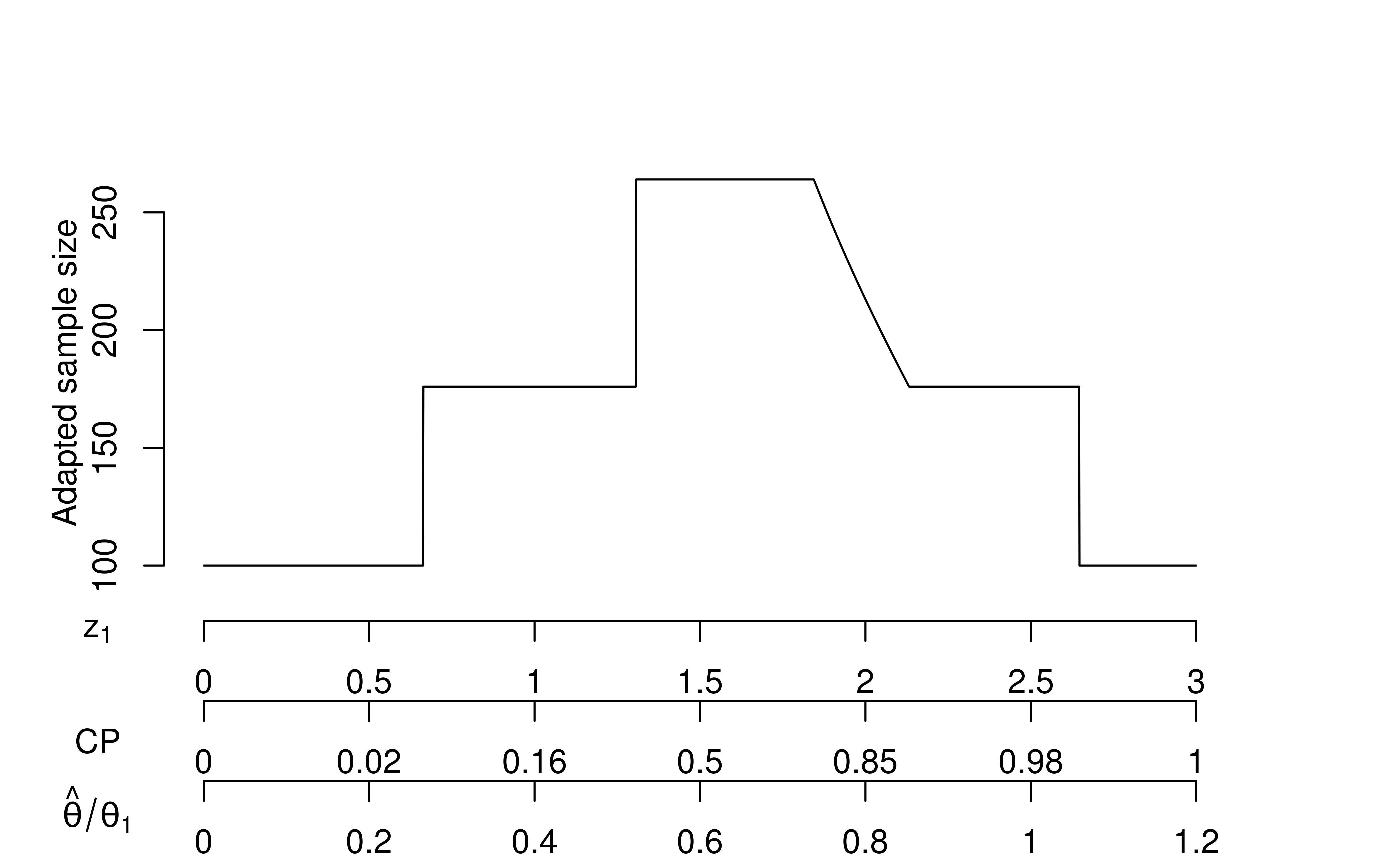

Figure 9.6: Stage 2 sample size plot, overlaid with densities for $Z$-values at IA1 under different hypotheses.

In Figure 9.6, you can see horizontal lines at sample size $N = 100$ where $Z_1$ is above the upper bound or below the lower bound at the interim analysis; in this case, we have just used the original group sequential design. We limit the sample size adaptation to a “promising” set of $Z_1$ values. Above the lower horizontal lines are horizontal lines at $N = 176$ where sample size is not adapted. For the smaller $Z_1$ values, no adaptation is done because the results are not promising enough. For the larger $Z_1$ values, the conditional power is at least the originally-planned 90% with the originally-planned final sample size. The sloped portion of the line denotes a region where the sample size is adapted to achieve 90% conditional power assuming the treatment effect observed at the interim analysis; a common complaint about this is that the interim treatment effect can be back-calculated if the adaptation algorithm is known in detail. The short horizontal line at $N = 264$ is a region where the results are promising, but increasing the sample size by more than a factor of 1.5x would be required to reach the targeted conditional power.

Now examine the three x-axes at the bottom of the graph.

There is a direct translation of $Z_1$ values to conditional power (CP) and, asymptotically, to the observed interim effect size relative to the effect size for which the trial is powered ($\hat{\theta}/\theta_1$). Thus, the sample size adaptation can be considered to be based on any one of these values. The Chen, DeMets, and Lan (2004) method does not adapt until conditional power is at least 0.5 which and thus the lower value for cadj is recommended to be 0.5 when z2 = z2Z (final test is unweighted).

9.6.2 Information-based sample size adaptation

We consider sample size adaptation based on estimating the variance of the treatment effect at the interim analysis. Note that statistical information is one over the variance of the treatment effect estimate. An information-based design examines statistical information instead of sample size at each analysis. We plan the analysis based on the treatment effect that we wish to detect, which was a difference of 2 in the means of the two treatment groups in this case (delta = delta1 = 2 below).

xI <- gsDesign(k = 2, delta = 2, delta1 = 2)
gsBoundSummary(
  xI,
  # Label for "sample size"
  Nname = "Information",
  # Digits for information on the left
  tdigits = 2
)
#>           Analysis               Value Efficacy Futility
#>          IA 1: 50%                   Z   2.7500   0.4122
#>  Information: 1.37         p (1-sided)   0.0030   0.3401
#>                        ~delta at bound   2.3496   0.3522
#>                    P(Cross) if delta=0   0.0030   0.6599
#>                    P(Cross) if delta=2   0.3412   0.0269
#>              Final                   Z   1.9811   1.9811
#>  Information: 2.74         p (1-sided)   0.0238   0.0238
#>                        ~delta at bound   1.1969   1.1969
#>                    P(Cross) if delta=0   0.0239   0.9761
#>                    P(Cross) if delta=2   0.9000   0.1000

Recall that we previously computed the standard error of the interim estimate of the difference of means and stored it in sedelta1. The inverse of the square of this is, thus, the statistical information at the interim analysis.

# Within group estimated standard deviation
sdhat1
#> [1] 5.2
# Sample size per group
npergroup <- xa$n.I[1] / 2
# Compute standard error for estimated difference in means
sedelta1 <- sqrt(sdhat1^2 * 2 / npergroup)

info1 <- 1 / sedelta1^2
info1
#> [1] 0.9245562

This is less than was planned for this case:

xI$n.I[1]
#> [1] 1.369775

We began using the sample sizes provided in the updated design stored in xa. Using the interim sample size there and the ratio of information observed at the interim compared to what is required at the final analysis, we can estimate the final sample size required to get final planned information. Note that we are getting an integer number per group and doubling from the original design:

# Proportion of targeted information at IA
t_ia <- info1 / xI$n.I[2]
t_ia
#> [1] 0.3374847

Now we increase final sample size per group estimated to get final information fraction of 1.

# Total planned adapted sample size
# Round up within each group
n2 <- 2 * ceiling(96 / t_ia / 2)
n2
#> [1] 286

Now we move on to the final analysis and suppose final within group standard deviation observed is 5; based on this we compute the final statistical information observed:

# Sample size per group
npergroup <- n2 / 2
# Within group standard deviation at final
sdhat2 <- 5
# Compute standard error for estimated difference in means
sedelta2 <- sqrt(sdhat2^2 * 2 / npergroup)

info2 <- 1 / sedelta2^2
info2
#> [1] 2.86

Based on the interim and final statistical information, we update the planned information-based design. Note that we could have done this calculation at the interim analysis based on an assumption for the final statistical information; the interim updated bounds would be the same as those computed here:

xIBD <- gsDesign(
  k = 2,
  # Targeted effect size
  delta = 2, delta1 = 2,
  # Max planned information
  maxn.IPlan = xI$n.I[2],
  n.I = c(info1, info2),
)
gsBoundSummary(
  xIBD,
  # Label for "sample size"
  Nname = "Information",
  # Digits for information on the left
  tdigits = 2
)
#>           Analysis               Value Efficacy Futility
#>          IA 1: 34%                   Z   3.0039  -0.2447
#>  Information: 0.92         p (1-sided)   0.0013   0.5967
#>                        ~delta at bound   3.1241  -0.2545
#>                    P(Cross) if delta=0   0.0013   0.4033
#>                    P(Cross) if delta=2   0.1399   0.0151
#>              Final                   Z   1.9727   1.9727
#>  Information: 2.86         p (1-sided)   0.0243   0.0243
#>                        ~delta at bound   1.1665   1.1665
#>                    P(Cross) if delta=0   0.0243   0.9757
#>                    P(Cross) if delta=2   0.9137   0.0863

Now we compute the final $Z$-statistic based on assuming an observed treatment difference of 1.5:

z2 <- 1.5 * sqrt(info2)
z2
#> [1] 2.53673

Since 2.54 is greater than the adjusted final efficacy bound of 1.97 computed just above (in xIBD$upper$bound), the null hypothesis can be rejected.

9.7 Information-based adaptation for a binomial design

9.7.1 Overview

The example we will develop here is a trial with a binomial outcome where the control group event rate is not known, and we wish to power the trial for a particular relative risk regardless of the control rate.

This is, by far, the most complex section of the book. It may be skipped by most, but may provide a useful example for others.

9.7.2 Basic strategy

Information-based design can be done blinded or unblinded, but there may be some preference from regulators that it be done on a blinded basis to ensure that those adapting, presumably a statistician from the trial sponsor, will not be taking into account treatment effect when updating the sample size. Even if somebody independent of the sponsor does the adaptation, there may be some possibility for back-calculation of the treatment effect observed if unblinded sample size adaptation is used.

The basic design strategy for adapting the sample size is as follows:

Design the study under an assumed value for the nuisance parameter.
At each interim analysis, compute an estimate of the nuisance parameter and update the statistical information, study bounds and sample size appropriately.

Following is the specific sample size adaptation strategy at each analysis, slightly modified from Zhou et al. (2014):

If current sample size is enough, meaning the planned final statistical information has been acquired, stop the trial regardless of whether efficacy or futility bound is crossed.
Otherwise, if overrun of patients enrolled between the analysis cutoff and performance of the analysis is enough to provide the planned final statistical information, stop enrolling more patients but keep collecting data for enrolled patients.
Otherwise, if the next planned sample size is enough, stop enrollment when that sample size is achieved.
Otherwise, if the next planned sample size is not enough but the overrun likely at the next interim would provide more than the planned final statistical information, stop at the estimated overrun. This will normally provide a little more than the planned information to be a bit conservative.
Otherwise, if the next planned sample size is not enough, but the original maximum sample size is, continue enrollment to the next planned interim.
Otherwise, if the original maximum sample size is not enough, use the updated maximum sample size but with an upper limit depending on practical aspects of certain trials (e.g., two times the originally planned maximum sample size) and continue enrollment to the next analysis.

9.7.3 The design and planned information

The design is loosely based on the CAPTURE study (The CAPTURE Investigators 1997) where abciximab was studied to reduce important cardiovascular outcomes following balloon angioplasty. The design assumed a control event rate of 15% and was powered at 80% to detect a 1/3 reduction to a 10% event rate in the experimental group. For this example, we assume 2.5%, one-sided Type I error and use default Hwang-Shih-DeCani bounds with $\gamma = -8$ for efficacy and $\gamma = -4$ for futility. Following is the code that is generated by the web interface for this trial:

# Derive binomial fixed design
n <- nBinomial(
  p1 = 0.15,
  p2 = 0.1,
  delta0 = 0,
  alpha = 0.025,
  beta = 0.2,
  ratio = 1
)

# Derive group sequential design
x <- gsDesign(
  k = 4,
  test.type = 4,
  alpha = 0.025,
  beta = 0.2,
  timing = c(1),
  sfu = sfHSD,
  sfupar = c(-8),
  sfl = sfHSD,
  sflpar = c(-4),
  delta = 0,
  delta1 = 0.05,
  delta0 = 0,
  endpoint = "binomial",
  n.fix = n
)

Figure 9.7 shows the resulting design with a planned sample size of 1469 and 3 equally-spaced interim analyses.

plot(x)

Figure 9.7: Boundaries plot for the design loosely based on the CAPTURE study.

As noted, we wish to be able to power the trial for a relative risk of 2/3, e.g., to a 10% experimental group event rate when the control rate is 15% or an 8% experimental group event rate when the control rate is 12%. For relative risk, the logarithm of the relative risk is used as the parameter of interest: $\delta = -\log(2/3)$. We used minus the logarithm so that $\delta$ is positive. If we used the same design parameters, but different control rates, we would get sample sizes as follows:

# Compute ratio of group sequential to
# fixed design sample size above
Inflate <- x$n.I[4] / n

# Compute fixed design sample sizes for different control rates
p1 <- seq(0.08, 0.2, 0.01)
nalt <- nBinomial(
  p1 = p1,
  p2 = p1 * 2 / 3,
  alpha = 0.025,
  beta = 0.2
)
df <- data.frame(x = p1, y = nalt * Inflate)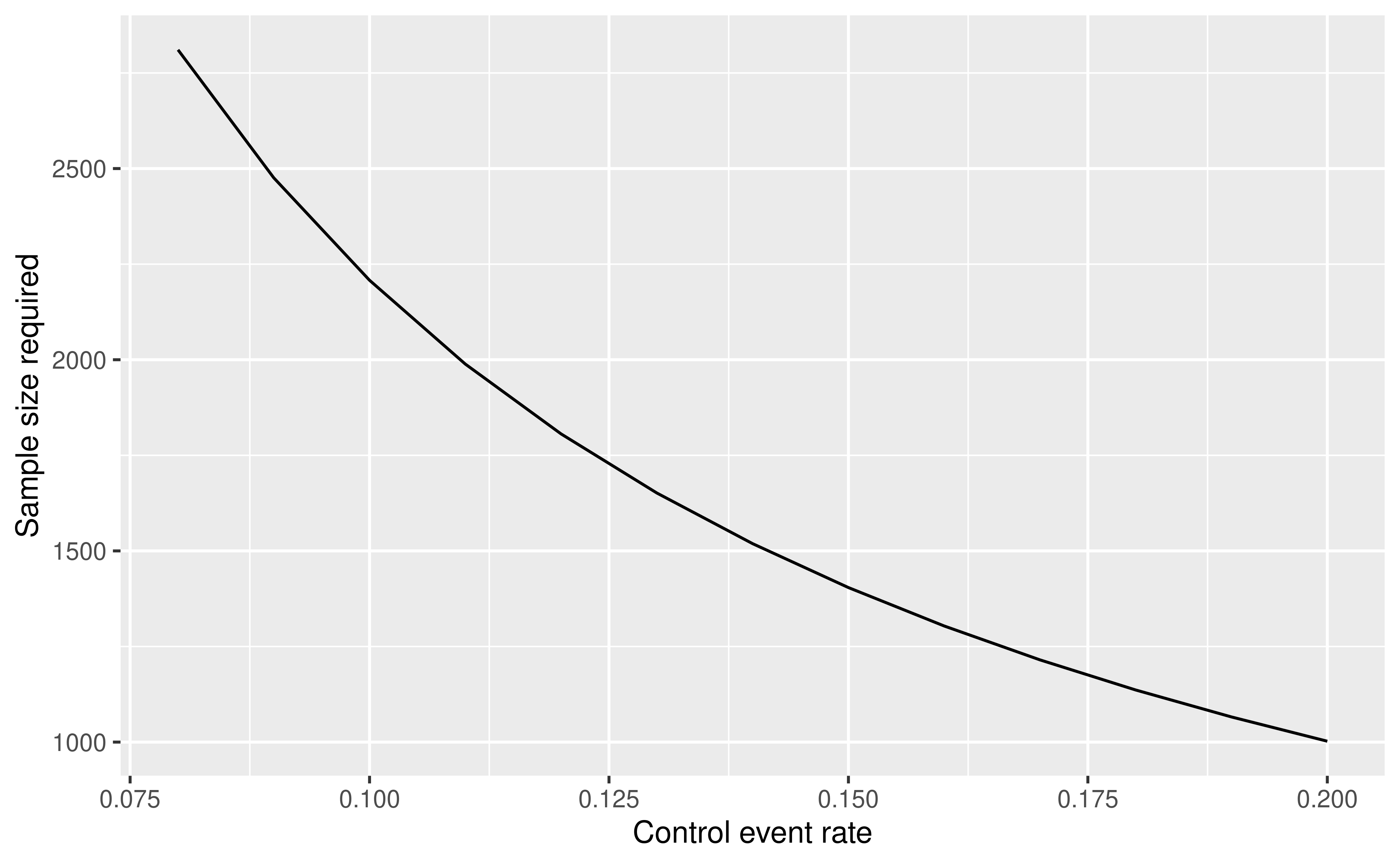

# Plot sample sizes using inflation factor and ggplot2
library(ggplot2)

ggplot(df, aes(x = x, y = y)) +
  geom_line() +
  xlab("Control event rate") +
  ylab("Sample size required")

Figure 9.8: Sample size required under different control rates.

Thus, you can see in Figure 9.8 that our sample size can vary from 1048 to almost 2940 depending on the value of the nuisance parameter. We will initially plan to do an analysis of the first 368 patients for interim 1 and adapt from there.

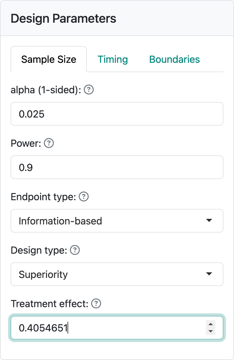
In the web interface, we can get the information-based design by entering $\delta$ = $-\log(2/3) = 0.4054651$ into the “Treatment effect” control (Figure 9.9).

Figure 9.9: Deriving the design using negative logarithm of the relative risk as “treatment effect” with information-based design in the web interface.

Deleting a couple of unnecessary parameters from the code generated, we re-derive a design with the same bounds, but on the information scale. x$n.I shows the resulting planned statistical information at each analysis.

# Derive group sequential design
x <- gsDesign(
  k = 4,
  test.type = 4,
  alpha = 0.025,
  beta = 0.2,
  timing = 1,
  sfu = sfHSD,
  sfupar = -8,
  sfl = sfHSD,
  sflpar = -2,
  delta = 0.4054651,
  delta1 = 0.4054651,
  delta0 = 0,
  endpoint = "info"
)
x$n.I
#> [1] 12.77867 25.55734 38.33600 51.11467

The plot for the bounds is now shown in Figure 9.10.

plot(x)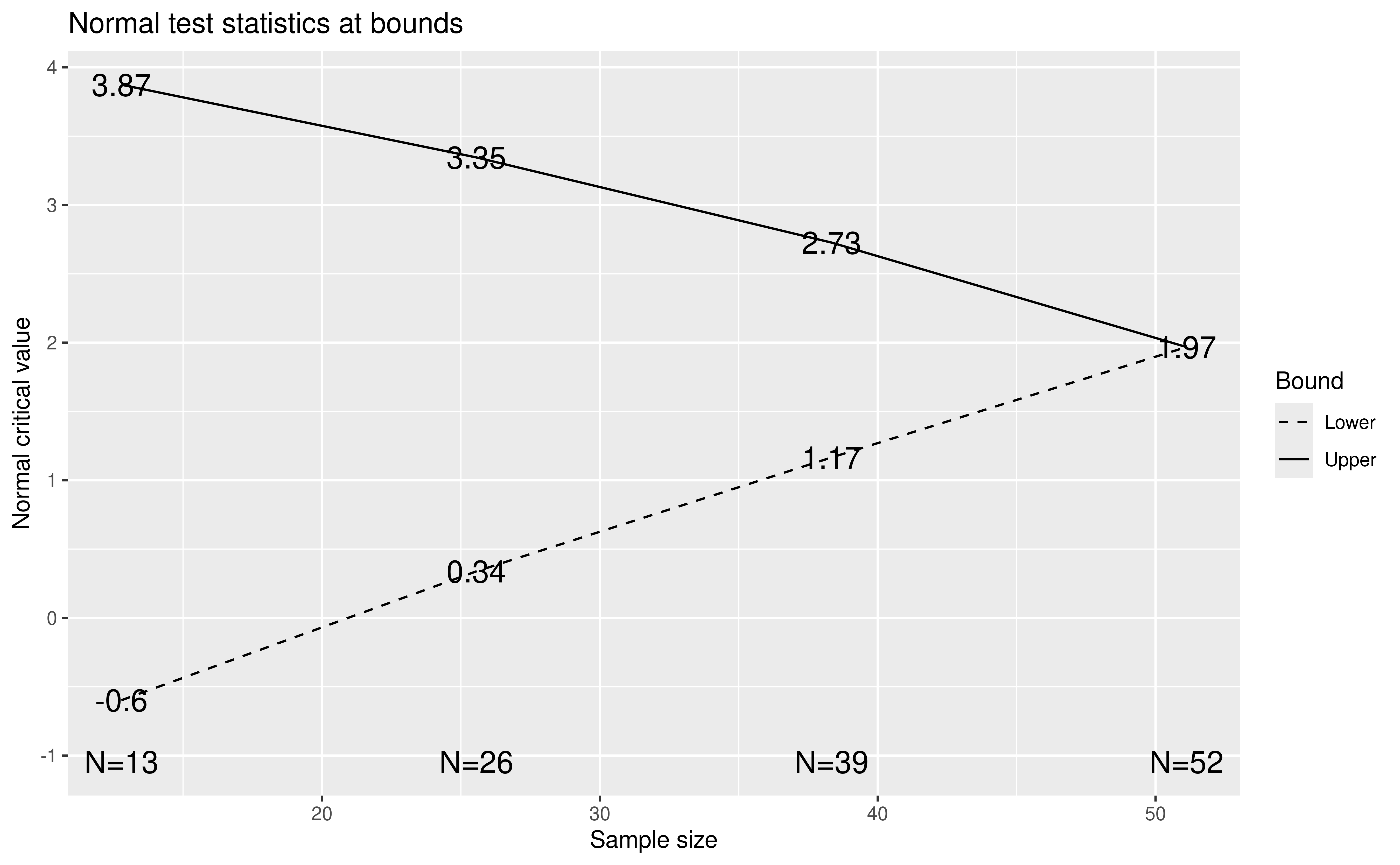

Figure 9.10: Boundaries plot for the re-derived design: same bounds but on the information scale.

9.7.4 Sample size adaptation

We will give an example of how the adaptation would have proceeded. We use a large control event rate which leads to a smaller sample size and keeps the example short. Following the basic strategy we have laid out we assume the first two analyses result in continuing the trial and adapting bounds. We assume 368 are patients included in the first interim with an equal number of 184 patients in each arm. On a blinded basis, we assume 67 events (18.2%) at interim 1. We can compute the estimated statistical information based on blinded data using the function varBinomial() as follows:

1 / varBinomial(
  x = 67,
  n = 368,
  scale = "RR"
)
#> [1] 20.47841

The above information calculation is under the null hypothesis. This is slightly different from under the alternative hypothesis:

1 / varBinomial(
  x = 67,
  n = 368,
  scale = "RR",
  delta0 = -log(2 / 3)
)
#> [1] 19.48577

Computing under either assumption has been adequate in simulations performed. We will use the alternate hypothesis calculation here which assumes that the observed event rate in the experimental group is 2/3 of that in the control group. The proportion of final planned information we have indicates a final sample size of needed to obtain the planned information is 966, rounding up to an even sample size, based on the following:

# Divide IA1 information by final planned information
relinf <- 1 / varBinomial(
  x = 67,
  n = 368,
  scale = "RR",
  delta0 = -log(2 / 3)
) / x$n.I[4]
368 / relinf
#> [1] 965.3298

This is about half-way between the planned second ($n = 736$) and third interims ($n = 1102$). Assuming an overrun of about 280 patients would occur by the time the $n = 736$ patients were enrolled, we plan to enroll to $n = 1016 = 736 + 280$ patients for the final analysis. This is slightly more than the estimated $n = 966$ needed, but is used here to provide a “cushion” to ensure an adequate sample size since the information at the final analysis is estimated based on the overall event rate remaining unchanged.

We will come back to the interim and final testing bounds momentarily, but assume that no bound is crossed at the interim. We assume that at the final sample size of 1016 that we observe 183 events for an event rate of 18%. The statistical information at this analysis is now computed as

1 / varBinomial(
  x = 183,
  n = 1016,
  scale = "RR",
  delta0 = -log(2 / 3)
)
#> [1] 53.10206

In spite of having a little lower event rate than at the interim, we still have more than the planned information ($53.10 > 51.11$).

We now update the code for the information-based design above based on the observed information at the two analyses above:

# Update design based on observed information
y <- gsDesign(
  k = 2,
  test.type = 4,
  alpha = 0.025,
  beta = 0.2,
  delta = 0.4054651,
  sfu = sfHSD,
  sfupar = -8,
  sfl = sfHSD,
  sflpar = -2,
  maxn.IPlan = x$n.I[4],
  n.I = c(20.47841, 53.10206)
)

In the above derivation of the updated design in y, we have just copied arguments for test.type, alpha, beta, delta, sfu, sfupar, sfl, and sflpar from what was provided by the web interface for computing the original design stored in x. Enter ?gsDesign in the console for more information on what is going on here. The new arguments here are maxn.IPlan which is the maximum planned sample size from the original design x and the information at the two analyses provided in the argument n.I. You can also see ?sfHSD for documentation of the Hwang-Shih-DeCani spending functions used. To see the updated design, we use plot(y); note that the information is rounded up here (Figure 9.11):

plot(y)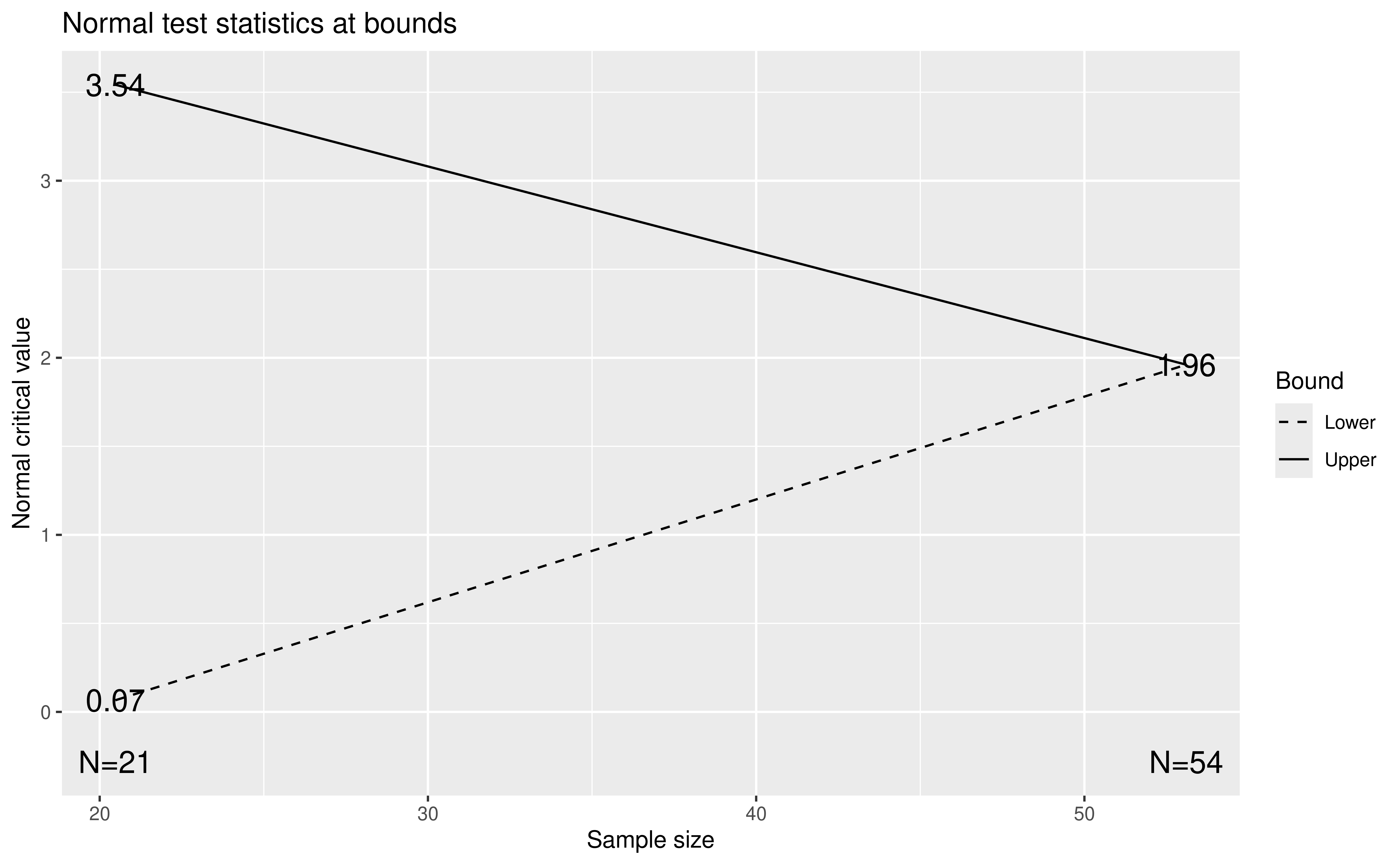

Figure 9.11: Boundaries plot of the updated design.

9.7.5 Testing and confidence intervals

We assume at the first analysis we have 184 patients per treatment group and that the total of 67 events is divided into 40 in the control group and 27 in the experimental group. The test statistic and repeated confidence interval for this difference is computed below. The repeated confidence interval method is described by Jennison and Turnbull (2000) for details. Basically, we use the $Z$-statistic for the efficacy bound at interim 1 and plug the corresponding confidence level into the function ciBinomial(). ciBinomial() computes confidence intervals for 1) the difference between two rates, 2) the risk-ratio for two rates, or 3) the odds-ratio for two rates. This procedure provides inference that is consistent with testBinomial() in that the confidence intervals are produced by inverting the testing procedures in testBinomial(). The testing and confidence interval calculations are as described in Miettinen and Nurminen (1985). The Type I error alpha input to ciBinomial() is always interpreted as 2-sided.

testBinomial(
  x1 = 40,
  n1 = 184,
  x2 = 27,
  n2 = 184
)
#> [1] 1.756089

level <- 2 * pnorm(-y$upper$bound[1])
ciBinomial(
  alpha = level,
  x1 = 27,
  n1 = 184,
  x2 = 40,
  n2 = 184,
  scale = "RR"
)
#>       lower    upper
#> 1 0.3065992 1.467228

This $Z = 1.76$ is between the efficacy ($z = 3.54$) and futility ($Z = 0.07$), so the trial continues. At the second, final analysis we assume equal sample sizes of 508 per arm and that the total of 183 events is divided between 108 in the control group and 75 in the experimental group. We compute the test statistic as

testBinomial(
  x1 = 108,
  n1 = 508,
  x2 = 75,
  n2 = 508
)
#> [1] 2.694094

which exceeds the final efficacy bound of 1.96, yielding a positive efficacy finding at the final analysis. In this case, the conservative spending functions yielded a final boundary of 1.961 compared to a bound of 1.960 if a fixed design had been used.

9.7.6 Alternate example

In the example above, we have also reduced the overall sample size needed from 1470 under the original assumption of a 15% control group event rate to 1016, a substantial savings. Note that if the overall event rate had been lower, a larger final sample size would have been suggested. Let’s test an example assuming that the low overall event rate is due to a larger than expected treatment effect.

We assume that after 184 per treatment group we have 28 events in the control group (15.2%) and 14 events (7.6%) in the experimental group. After 368 per treatment group we have 58 events in the control group (15.8%) and 27 events (7.3%) in the experimental group. This yields the following adaptation and positive efficacy finding at the second interim analysis:

# Compute information after IA's 1 and 2
info <- 1 / c(
  varBinomial(
    x = 42, n = 368, scale = "RR", delta0 = -log(2 / 3)
  ),
  varBinomial(
    x = 85, n = 736, scale = "RR", delta0 = -log(2 / 3)
  )
)
info
#> [1] 11.32031 22.94377

# After IA2, compute estimated maximum sample size needed
relinfo <- info[2] / 51.11
nupdate <- 736 / relinfo
nupdate
#> [1] 1639.529

# Update design based on observed information at IA1 and
# assumed final information
y <- gsDesign(
  k = 2,
  test.type = 4,
  alpha = 0.025,
  beta = 0.2,
  delta = 0.4054651,
  sfu = sfHSD,
  sfupar = -8,
  sfl = sfHSD,
  sflpar = -2,
  maxn.IPlan = x$n.I[4],
  n.I = info
)

# Compute Z-values for IA's 1 and 2
testBinomial(
  x1 = c(28, 58),
  n1 = c(184, 368),
  x2 = c(14, 27),
  n2 = c(184, 368)
)
#> [1] 2.295189 3.575202

# Compare above to updated IA1 and IA2 efficacy bounds
y$upper$bound
#> [1] 3.938772 3.465813

We see that the updated sample size based on blinded data would be 1662. However, you can see that the second interim $Z = 3.58$ is greater than the efficacy bound of 3.47 and thus the trial can stop for a positive efficacy finding at that point. Assuming there is an overrun of 280 patients as before, we again end with a final sample size of 1016, a savings compared to the planned maximum sample size. In combination, the two examples show a couple of ways that the trial can adapt to produce savings compared to the planned sample size of 1470.