13 Exact binomial group sequential designs
Exact binomial methods are useful when the number of events is small and normal approximations may not be reliable. This arises frequently in vaccine efficacy trials, where a highly effective vaccine leads to few endpoint cases, and in single-arm safety or response rate monitoring. The gsDesign package provides gsBinomialExact() for exact boundary crossing probabilities under a binomial model and binomialSPRT() for deriving truncated sequential probability ratio test (SPRT) bounds. The toBinomialExact() function bridges the asymptotic time-to-event design framework with exact binomial calculations, enabling spending-function-based boundary derivation.
13.1 Vaccine efficacy trial design
This section explores a method of approximating a design using the exact binomial method of Chan and Bohidar (1998) by a time-to-event design using the method of Lachin and Foulkes (1986). This allows use of spending functions to derive boundaries for the exact method. The time-to-event design not only sets boundaries for the Chan and Bohidar (1998) method but also allows specification of enrollment duration and study duration to determine enrollment rates and sample size. This section also illustrates the concept of super-superiority often used in prevention studies.
13.1.1 Parameterization
We begin with the assumption of a large sample size due to an endpoint with a small incidence rate, as in a vaccine study or other prevention study with a relatively small number of events expected.
Paralleling the notation of Chan and Bohidar (1998), we assume \(N_C, P_C\) to be binomial sample size and probability of an event for each participant assigned to control; for the experimental treatment group, these are \(N_E, P_E\). Vaccine efficacy is defined as
\[\pi = 1 - P_E/P_C.\]
The parameter \(\pi\) is often labeled as VE for vaccine efficacy. Taking into account the randomization ratio \(r\) (experimental/control), the approximate probability that any given event is in the experimental group is
\[ p = \frac{r}{r + (1-\pi)^{-1}}. \]
This approximation is dependent on a large sample size and small probability of events. The above can be inverted to obtain
\[\pi = 1 - \frac{1}{r(1/p-1)}.\]
For an example with alternate hypothesis vaccine efficacy \(\pi_1 = 0.7\) and experimental:control randomization ratio \(r = 3\):
pi1 <- .7
ratio <- 3
p1 <- ratio / (ratio + 1 / (1 - pi1))
p1
#> [1] 0.4736842
The inversion formula recovers \(\pi_1 = 0.7\):
1 - 1 / (ratio * (1 / p1 - 1))
#> [1] 0.7
With null hypothesis vaccine efficacy \(\pi_0 = 0.3\), the null hypothesis probability that an event is in the experimental group is:
pi0 <- .3
p0 <- ratio / (ratio + 1 / (1 - pi0))
p0
#> [1] 0.6774194
We also translate several vaccine efficacy values to proportion of events in the experimental group:
ve <- c(.5, .6, .65, .7, .75, .8)
prob_experimental <- ratio / (ratio + 1 / (1 - ve))
tibble::tibble(VE = ve, "P(Experimental)" = prob_experimental) |>
  gt() |>
  tab_options(data_row.padding = px(1)) |>
fmt_number(columns = 2, decimals = 3)| VE | P(Experimental) |
|---|---|
| 0.50 | 0.600 |
| 0.60 | 0.545 |
| 0.65 | 0.512 |
| 0.70 | 0.474 |
| 0.75 | 0.429 |
| 0.80 | 0.375 |
13.1.2 The time-to-event approximation
For a time-to-event formulation with exponential failure rates \(\lambda_C\) for control and \(\lambda_E\) for experimental group, vaccine efficacy is
\[\pi = 1 - \lambda_E / \lambda_C\]
which is 1 minus the hazard ratio. The time-to-event method using asymptotic distributional assumptions can approximate an appropriate exact binomial design while also providing sample size and study duration estimates not given by the exact binomial approach alone.
We specify design parameters:
alpha <- 0.025
beta <- 0.1
k <- 3
timing <- c(.45, .7)
sfu <- sfHSD
sfupar <- -3
sfl <- sfHSD
sflpar <- -3
failRate <- .002
dropoutRate <- .0001
enrollDuration <- 8
trialDuration <- 24
VE1 <- .7
VE0 <- .3
ratio <- 3
test.type <- 4
Now we generate the time-to-event design, translating vaccine efficacy to hazard ratio:
x <- gsSurv(
  k = k, test.type = test.type, alpha = alpha, beta = beta,
  timing = timing,
  sfu = sfu, sfupar = sfupar, sfl = sfl, sflpar = sflpar,
  lambdaC = failRate, eta = dropoutRate,
  hr = 1 - VE1, hr0 = 1 - VE0,
  R = enrollDuration, T = trialDuration,
  minfup = trialDuration - enrollDuration, ratio = ratio
)
Converting to integer event counts at analyses:
xx <- toInteger(x)
gsBoundSummary(xx,
  tdigits = 1, logdelta = TRUE, deltaname = "HR", Nname = "Events",
  exclude = c("B-value", "CP", "CP H1", "PP")
) |>
  gt() |>
  tab_header(
    title = "Initial group sequential approximation",
    subtitle = "Integer event counts at analyses"
  ) |>
tab_options(data_row.padding = px(1))| Initial group sequential approximation | |||
| Integer event counts at analyses | |||
| Analysis | Value | Efficacy | Futility |
|---|---|---|---|
| IA 1: 46% | Z | 2.6664 | 0.1028 |
| Events: 3632 | p (1-sided) | 0.0038 | 0.4591 |
| Events: 31 | ~HR at bound | 0.2316 | 0.6708 |
| Month: 13 | Spending | 0.0038 | 0.0153 |
| P(Cross) if HR=0.7 | 0.0038 | 0.5409 | |
| P(Cross) if HR=0.3 | 0.3438 | 0.0153 | |
| IA 2: 71% | Z | 2.4301 | 0.9679 |
| Events: 3632 | p (1-sided) | 0.0075 | 0.1665 |
| Events: 48 | ~HR at bound | 0.3114 | 0.5070 |
| Month: 18.1 | Spending | 0.0057 | 0.0230 |
| P(Cross) if HR=0.7 | 0.0096 | 0.8419 | |
| P(Cross) if HR=0.3 | 0.6635 | 0.0383 | |
| Final | Z | 2.0322 | 2.0322 |
| Events: 3632 | p (1-sided) | 0.0211 | 0.0211 |
| Events: 68 | ~HR at bound | 0.3962 | 0.3962 |
| Month: 24 | Spending | 0.0154 | 0.0617 |
| P(Cross) if HR=0.7 | 0.0239 | 0.9761 | |
| P(Cross) if HR=0.3 | 0.9018 | 0.0982 | |
A textual summary for the design is:
Asymmetric two-sided group sequential design with non-binding futility bound, 3 analyses, time-to-event outcome with sample size 3632 and 68 events required, 90 percent power, 2.5 percent (1-sided) Type I error to detect a hazard ratio of 0.3 with a null hypothesis hazard ratio of 0.7. Enrollment and total study durations are assumed to be 8 and 24 months, respectively. Efficacy bounds derived using a Hwang-Shih-DeCani spending function with gamma = -3. Futility bounds derived using a Hwang-Shih-DeCani spending function with gamma = -3.
13.1.3 Converting to an exact binomial design
We now convert this to an exact binomial design using toBinomialExact(). The efficacy bound a is the maximum number of events in the experimental group to cross the efficacy bound. The futility bound b is the minimum number of experimental group events to cross the futility bound. Because fewer experimental-group events support vaccine efficacy, a is stored in lower$bound, while b is stored in upper$bound.
xb <- toBinomialExact(x)The initial approximation of bounds uses the nominal p-values from the asymptotic design:
efficacyNominalPValue <- pnorm(-xx$upper$bound)
efficacyNominalPValue
#> [1] 0.003832879 0.007548194 0.021066070
Applying the inverse binomial distribution:
qbinom(p = efficacyNominalPValue, size = xx$n.I, prob = p0) - 1
#> [1] 13 23 37
These match the final efficacy bounds:
xb$lower$bound
#> [1] 13 24 37
The initial approximation and final futility bounds:
xb$init_approx$a
#> [1] 13 23 37
xb$init_approx$b
#> [1] 21 29 38
xb$upper$bound
#> [1] 22 30 38
13.1.4 Checking design properties
For both \(\alpha\)- and \(\beta\)-spending, the exact binomial design should have no more spending at each analysis than allowed by the spending function. We also confirm that changing any bound by 1 exceeds the targeted spending.
13.1.4.1 Alpha-spending
# Exact design cumulative alpha-spending (non-binding)
nb <- gsBinomialExact(
  k = xb$k, theta = xb$theta, n.I = xb$n.I,
  b = xb$n.I + 1, a = xb$lower$bound
)
cumsum(nb$lower$prob[, 1])
#> Analysis  1 Analysis  2 Analysis  3
#> 0.002703239 0.009176778 0.018982186
# Targeted alpha-spending
xx$upper$sf(alpha, t = xx$timing, xx$upper$param)$spend
#> [1] 0.003832879 0.009577354 0.025000000
Increasing any efficacy bound by 1 exceeds the targeted cumulative spend:
excess_alpha_spend <- matrix(0, nrow = nb$k, ncol = nb$k)
for (i in 1:xb$k) {
  a <- xb$lower$bound
  a[i] <- a[i] + 1
  excess_alpha_spend[i, ] <-
    cumsum(gsBinomialExact(
      k = xb$k, theta = xb$theta, n.I = xb$n.I,
      b = xb$n.I + 1, a = a
    )$lower$prob[, 1])
}
excess_alpha_spend
#>             [,1]        [,2]       [,3]
#> [1,] 0.007742914 0.012745616 0.02201467
#> [2,] 0.002703239 0.017820794 0.02502423
#> [3,] 0.002703239 0.009176778 0.02967058
13.1.4.2 Beta-spending
# Cumulative beta-spending for exact design
cumsum(xb$upper$prob[, 2])
#> Analysis  1 Analysis  2 Analysis  3
#> 0.006760093 0.027359634 0.097411064
# Targeted beta-spending
xx$lower$sf(beta, t = xx$timing, xx$lower$param)$spend
#> [1] 0.01533151 0.03830942 0.10000000
Decreasing any interim futility bound by 1 exceeds targeted spending:
excess_beta_spend <- matrix(0, nrow = nb$k - 1, ncol = nb$k)
for (i in 1:(xb$k - 1)) {
  b <- xb$upper$bound
  b[i] <- b[i] - 1
  excess_beta_spend[i, ] <-
    cumsum(as.numeric(gsBinomialExact(
      k = xb$k, theta = xb$theta, n.I = xb$n.I,
      b = b, a = xb$lower$bound
    )$upper$prob[, 2]))
}
excess_beta_spend
#>             [,1]       [,2]      [,3]
#> [1,] 0.017842801 0.03386750 0.1009881
#> [2,] 0.006760093 0.04900921 0.1046241
Choosing the spending function carefully to ensure cumulative spending for the exact design is close to the targeted \(\alpha\) is worth careful examination.
13.1.5 Updating bounds at the time of analysis
When observed event counts differ from planned, bounds must be updated using the spending functions based on the altered information fraction. We illustrate with the second interim analysis from the SPUTNIK trial (Logunov et al. 2021), where 20 events were observed at the first database lock and 78 events one week later:
ebUpdate <- toBinomialExact(xx, observedEvents = c(20, 78))| Updated Bounds for Actual Analyses from SPUTNIK Trial | ||||||||||
| Analysis | Cases |
Cases at Bound1
|
VE at Bound2
|
Error Spending3
|
Power by VE4
|
|||||
|---|---|---|---|---|---|---|---|---|---|---|
| Success | Futility | Efficacy | Futility | alpha5 | beta | 65% | 75% | 85% | ||
| 1 | 20 | 6 | 16 | 0.86 | −0.33 | 0.0006 | 0.0030 | 0.05 | 0.18 | 0.57 |
| 2 | 78 | 44 | 45 | 0.57 | 0.55 | 0.0239 | 0.0450 | 0.85 | 0.99 | 1.00 |
| 1 Experimental case counts; counts between success and futility bounds do not stop trial | ||||||||||
| 2 Exact vaccine efficacy required to cross bound | ||||||||||
| 3 Cumulative spending at each analysis | ||||||||||
| 4 Cumulative power at each analysis by underlying vaccine efficacy | ||||||||||
| 5 Efficacy spending ignores non-binding futility bound | ||||||||||
At the time of analysis of 78 endpoint events, 16 were in the experimental group, comfortably crossing the efficacy bound requiring 44 or fewer experimental events. Since Type I error assumed a non-binding bound, the first analysis futility bound could be ignored for decision-making purposes without inflating Type I error.
13.2 Binomial SPRT
The sequential probability ratio test (SPRT) was proposed by Wald (1947) and Wald and Wolfowitz (1948) as a way to do continuous sampling to assess product quality. In clinical trials, the SPRT for a single-arm binary endpoint can be useful to raise or alleviate concerns about a short-term endpoint such as an important safety event or, for efficacy, a response rate.
The function binomialSPRT() implements a single-arm version of the SPRT for a binary outcome, truncated to a specified minimum and maximum sample size.
13.2.1 Response rate example
Consider a single arm where historical data suggests a positive response occurs in no more than 10% of patients, and there is interest in detecting a response rate of 35%. We assume a minimum sample size of 10, a maximum of 25, one-sided \(\alpha = 0.08\), and power of 80%:
b <- binomialSPRT(
  p0 = .1, p1 = .35, alpha = .08, beta = .2,
  minn = 10, maxn = 25
)
plot(b)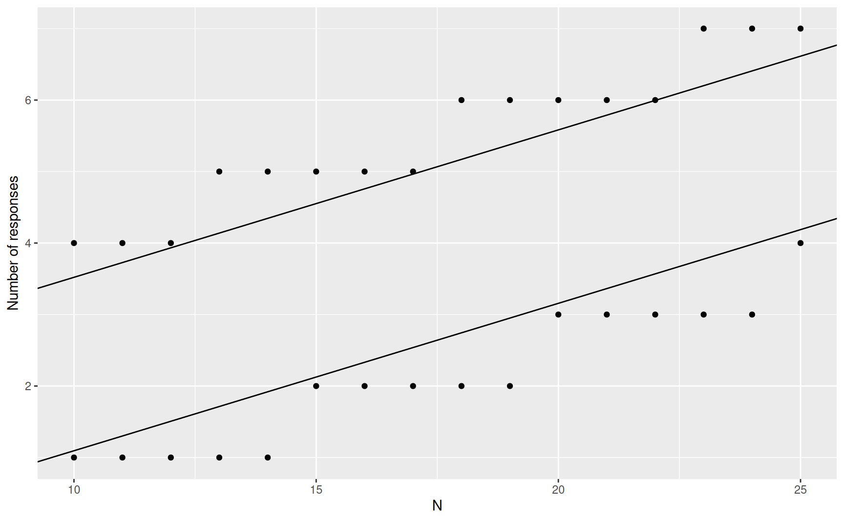
The plot tests first after 10 patients. If 4/10 have responded, the null hypothesis of a 10% response rate is rejected. If 0 or 1 of 10 have responded, we conclude that the targeted 35% response rate is not realistic. At the maximum sample size of 25:
- If 4 or fewer patients have responded, we accept the null hypothesis.
- If 7 or more patients have responded, we reject the null hypothesis.
- If 5 or 6 patients respond, the result is indeterminate.
A power plot summarizes the probability of each outcome by underlying response rate:
plot(b, plottype = 2)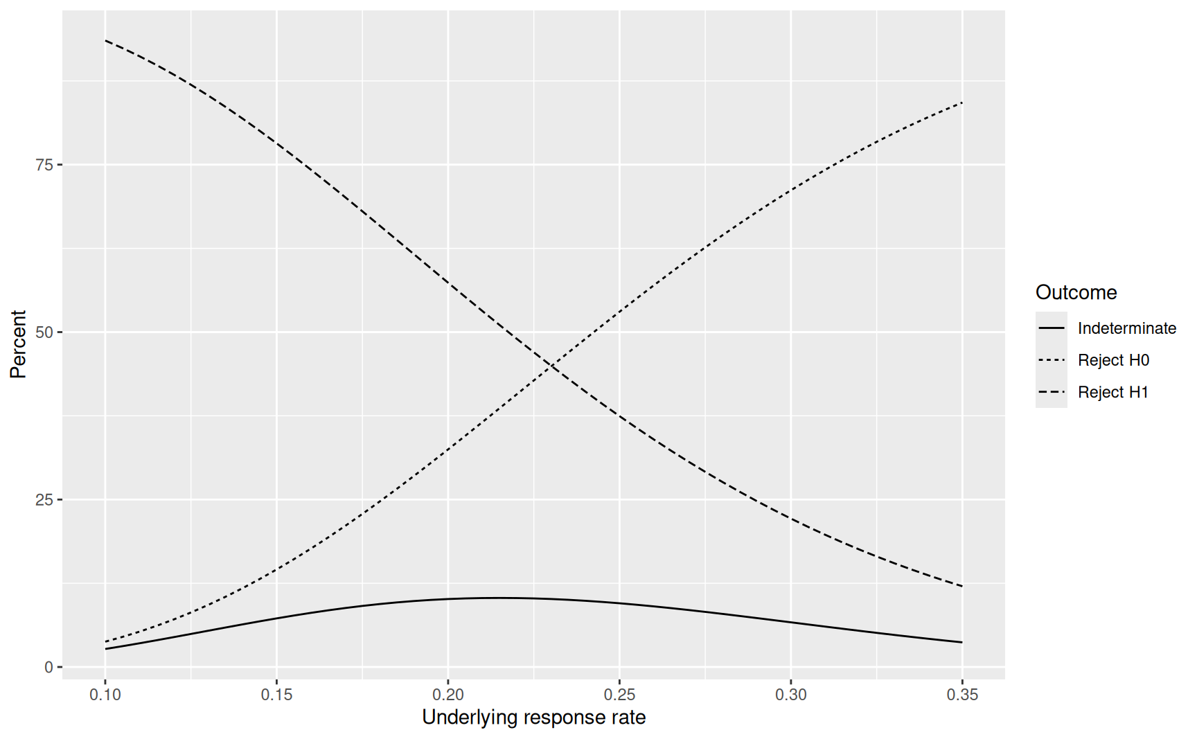
The three outcomes shown are:
- Solid line: Indeterminate outcome (no bound crossed). Probabilities are small, even for rates midway between the null and alternative.
- Short-dashed line: Reject \(H_0\). The actual Type I error is below the targeted \(\alpha = 0.08\) due to truncation.
- Long-dashed line: Reject \(H_1\). There is >90% chance of rejecting a 35% response rate if the true rate is 10%.
Operating characteristics can be summarized in a table using gsBinomialExact() to compute boundary crossing probabilities for selected response rates:
b_power <- gsBinomialExact(
  k = length(b$n.I), theta = seq(.1, .45, .05),
  n.I = b$n.I,
  a = b$lower$bound, b = b$upper$bound
)
b_power |>
  as_table() |>
as_gt()| Operating Characteristics for the Truncated SPRT Design | |||
| Assumes trial evaluated sequentially after each response | |||
| Underlying response rate |
Probability of crossing
|
Average sample size |
|
|---|---|---|---|
| Futility bound | Efficacy bound | ||
| 10% | 0.94 | 0.04 | 12.1 |
| 15% | 0.78 | 0.15 | 13.6 |
| 20% | 0.57 | 0.32 | 14.3 |
| 25% | 0.37 | 0.53 | 14.2 |
| 30% | 0.22 | 0.71 | 13.4 |
| 35% | 0.12 | 0.84 | 12.5 |
| 40% | 0.06 | 0.92 | 11.6 |
| 45% | 0.03 | 0.97 | 11.0 |
13.2.2 Safety monitoring example
Suppose a new treatment has potential for an elevated rate of a specific adverse experience (e.g., serious rash). This already occurs in the population at about 4% and a 10% rate would be considered unacceptable. With a proposed sample size of 75 per arm and no stopping before 4 patients in the experimental group:
safety_design <- binomialSPRT(
  p0 = .04, p1 = .1, alpha = .04, beta = .2,
  minn = 4, maxn = 75
)
plot(safety_design)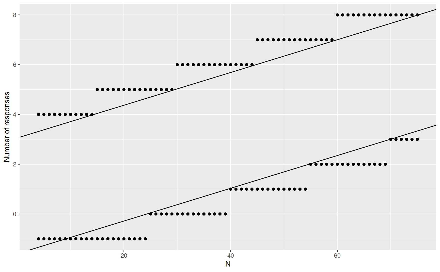
If the first 25 experimental patients have no serious rashes, or 1 in the first 40, we reject the 10% rate of concern. If the first 4 of the first 4–14 patients have serious rashes, we reject the null hypothesis that there is no elevation over the 4% population rate.
plot(safety_design, plottype = 2)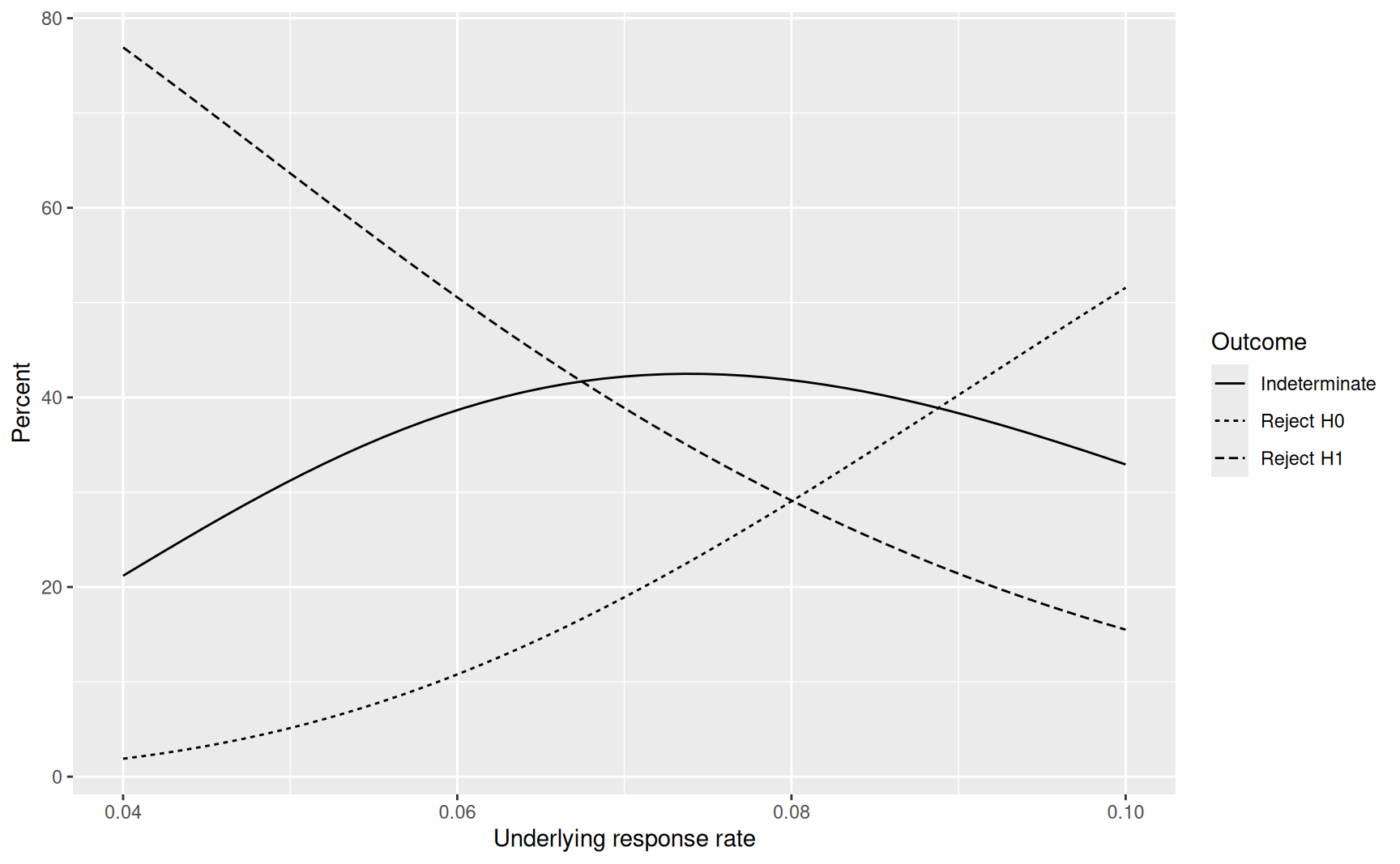
There can be a fairly high probability of an indeterminate outcome. Including more extreme rates in the summary shows the indeterminate probability decreasing:
safety_power <- gsBinomialExact(
  k = length(safety_design$n.I),
  theta = seq(.02, .16, .02),
  n.I = safety_design$n.I,
  a = safety_design$lower$bound,
  b = safety_design$upper$bound
)
safety_power |>
  as_table() |>
  as_gt(
    theta_label = gt::html("Underlying<br>AE rate"),
    prob_decimals = 3,
    bound_label = c("low rate", "high rate")
)| Operating Characteristics for the Truncated SPRT Design | |||
| Assumes trial evaluated sequentially after each response | |||
| Underlying AE rate |
Probability of crossing
|
Average sample size |
|
|---|---|---|---|
| low rate | high rate | ||
| 2% | 0.964 | 0.001 | 34.8 |
| 4% | 0.769 | 0.019 | 46.4 |
| 6% | 0.506 | 0.108 | 54.3 |
| 8% | 0.291 | 0.290 | 56.1 |
| 10% | 0.155 | 0.516 | 52.8 |
| 12% | 0.079 | 0.714 | 46.8 |
| 14% | 0.039 | 0.851 | 40.2 |
| 16% | 0.020 | 0.930 | 34.2 |
Note that sequential patients should be analyzed, but if you cross a high rate bound with some incomplete data included as safe, you can still declare that the bound was crossed since the number of adverse experience cases cannot go down when missing cases are filled in.