14 Design and simulation for negative binomial outcomes
Recurrent event endpoints — such as exacerbation counts in respiratory disease, relapse counts in multiple sclerosis, or infection episodes — are common in clinical trials. When individual event rates vary across patients, the negative binomial model provides a natural framework that accounts for this overdispersion. The gsDesignNB package (Anderson 2025) extends the gsDesign framework to support sample size calculation, group sequential design, and simulation for trials with negative binomial outcomes.
This chapter covers:
- The negative binomial distribution and its Gamma-Poisson mixture motivation.
- Fixed-design sample size calculation using the Zhu and Lakkis method (Zhu and Lakkis 2014).
- Handling variable accrual, dropout, maximum follow-up, and event gaps.
- Non-inferiority and super-superiority testing.
- Group sequential designs via
gsNBCalendar(). - Simulation of recurrent events and verification of design properties.
14.1 The negative binomial model
We assume the outcome \(Y\) follows a negative binomial distribution with mean \(\mu\) and a common dispersion parameter \(k\) for both treatment groups, such that the variance is
\[\text{Var}(Y) = \mu + k\mu^2.\]
Setting \(k = 0\) recovers the Poisson distribution. In R’s rnbinom parameterization, \(k = 1/\texttt{size}\).
14.1.1 Gamma-Poisson mixture motivation
The negative binomial arises naturally as a Gamma-Poisson mixture. For each subject \(i\), the individual event rate \(\Lambda_i\) follows a Gamma distribution with shape \(\alpha = 1/k\) and rate \(\beta = 1/(k\lambda)\), where \(\lambda\) is the population event rate:
\[\Lambda_i \sim \text{Gamma}(1/k, \; 1/(k\lambda))\]
Given the subject-specific rate, the number of events over exposure time \(t_i\) follows a Poisson distribution:
\[Y_i \mid \Lambda_i \sim \text{Poisson}(\Lambda_i t_i)\]
The marginal distribution of \(Y_i\) is then negative binomial with mean \(\mu_i = \lambda t_i\) and variance \(\text{Var}(Y_i) = \lambda t_i + k(\lambda t_i)^2\). This connects the event rate \(\lambda\) (used in hypothesis testing) with the expected count \(\mu\) (used in the negative binomial parameterization), showing how heterogeneity in individual rates leads to overdispersion.
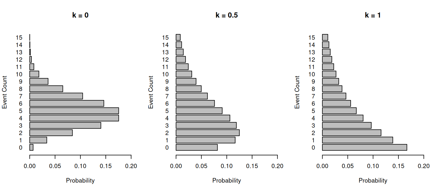
As \(k\) increases, the variance increases and the distribution spreads out:
par(mfrow = c(1, 3))
k_values <- c(0, 0.5, 1)
for (k in k_values) {
  mu <- 5
  x <- 0:15
  if (k == 0) {
    probs <- dpois(x, lambda = mu)
  } else {
    size <- 1 / k
    probs <- dnbinom(x, size = size, mu = mu)
  }
  barplot(probs,
    names.arg = x, horiz = TRUE, main = paste("k =", k),
    xlab = "Probability", ylab = "Event Count", las = 1, xlim = c(0, 0.2)
  )
}
14.2 Sample size calculation
The sample size calculation is based on the asymptotic normality of the log rate ratio, \(\theta = \log(\lambda_2/\lambda_1)\), corresponding to Method 3 of Zhu and Lakkis (2014) (Wald statistic on the log rate ratio). This is also the method described by Friede and Schmidli (2010) and Mütze et al. (2019).
The total sample size is
\[n_{\text{total}} = \frac{(z_{\alpha/s} + z_\beta)^2 \cdot \tilde{V}}{(\theta - \theta_0)^2}\]
where \(\theta_0\) is the log rate ratio under the null hypothesis (default 0 for superiority) and \(\tilde{V}\) is the average variance per subject:
\[\tilde{V} = \frac{1/\mu_1 + k_1}{p_1} + \frac{1/\mu_2 + k_2}{p_2}\]
with allocation proportions \(p_1, p_2\) and expected mean counts \(\mu_i = \lambda_i \bar{t}_i\) over the average exposure duration \(\bar{t}_i\).
14.2.1 Basic example
We calculate the sample size for a trial comparing event rates of \(\lambda_1 = 0.5\) (control) and \(\lambda_2 = 0.3\) (experimental) events per unit time, with dispersion \(k = 0.1\), 80% power, and one-sided \(\alpha = 0.025\):
The dispersion argument corresponds directly to \(k\) in \(\text{Var}(Y)=\mu+k\mu^2\); the equivalent R negative-binomial parameter is size = 1 / dispersion.
sample_size_nbinom(
  lambda1 = 0.5,
  lambda2 = 0.3,
  dispersion = 0.1,
  power = 0.8,
  alpha = 0.025,
  sided = 1,
  accrual_rate = 10,
  accrual_duration = 12,
  trial_duration = 12
)
#> Sample size for negative binomial outcome
#> ==========================================
#>
#> Sample size:     n1 = 35, n2 = 35, total = 70
#> Expected events: 168.0 (n1: 105.0, n2: 63.0)
#> Power: 80%, Alpha: 0.025 (1-sided)
#> Rates: control = 0.5000, treatment = 0.3000 (RR = 0.6000)
#> Dispersion: 0.1000, Avg exposure (calendar): 6.00
#> Accrual: 12.0, Trial duration: 12.0
14.2.2 Piecewise constant accrual
Recruitment often ramps up over time. The function handles piecewise constant accrual, automatically calculating the average exposure:
sample_size_nbinom(
  lambda1 = 0.5,
  lambda2 = 0.3,
  dispersion = 0.1,
  power = 0.8,
  accrual_rate = c(5, 10),
  accrual_duration = c(3, 3),
  trial_duration = 12
)
#> Sample size for negative binomial outcome
#> ==========================================
#>
#> Sample size:     n1 = 26, n2 = 26, total = 52
#> Expected events: 176.8 (n1: 110.5, n2: 66.3)
#> Power: 80%, Alpha: 0.025 (1-sided)
#> Rates: control = 0.5000, treatment = 0.3000 (RR = 0.6000)
#> Dispersion: 0.1000, Avg exposure (calendar): 8.50
#> Accrual: 6.0, Trial duration: 12.0
14.2.3 Dropout and maximum follow-up
Adding a 5% dropout rate per unit time and capping follow-up at 6 months:
sample_size_nbinom(
  lambda1 = 0.5,
  lambda2 = 0.3,
  dispersion = 0.1,
  power = 0.8,
  accrual_rate = c(5, 10),
  accrual_duration = c(3, 3),
  trial_duration = 12,
  dropout_rate = 0.05,
  max_followup = 6
)
#> Sample size for negative binomial outcome
#> ==========================================
#>
#> Sample size:     n1 = 38, n2 = 38, total = 76
#> Expected events: 157.6 (n1: 98.5, n2: 59.1)
#> Power: 80%, Alpha: 0.025 (1-sided)
#> Rates: control = 0.5000, treatment = 0.3000 (RR = 0.6000)
#> Dispersion: 0.1000, Avg exposure (calendar): 5.18
#> Dropout rate: 0.0500
#> Accrual: 6.0, Trial duration: 12.0
#> Max follow-up: 6.0
Group-specific dropout rates are also supported by providing a vector of length 2 (control, experimental):
sample_size_nbinom(
  lambda1 = 0.5,
  lambda2 = 0.3,
  dispersion = 0.1,
  power = 0.8,
  accrual_rate = c(5, 10),
  accrual_duration = c(3, 3),
  trial_duration = 12,
  dropout_rate = c(0.10, 0.05),
  max_followup = 6
)
#> Sample size for negative binomial outcome
#> ==========================================
#>
#> Sample size:     n1 = 40, n2 = 40, total = 80
#> Expected events: 152.4 (n1: 90.2, n2: 62.2)
#> Power: 80%, Alpha: 0.025 (1-sided)
#> Rates: control = 0.5000, treatment = 0.3000 (RR = 0.6000)
#> Dispersion: 0.1000, Avg exposure (calendar): 4.51 (n1), 5.18 (n2)
#> Dropout rate: 0.1000 (n1), 0.0500 (n2)
#> Accrual: 6.0, Trial duration: 12.0
#> Max follow-up: 6.0
14.2.4 Event gaps
In some recurrent event trials, there is a mandatory gap after each event during which no new events can occur (e.g., a recovery period). The function adjusts the effective event rate as
\[\lambda_{\text{eff}} \approx \frac{\lambda}{1 + \lambda \cdot \text{gap}}\]
and reports the at-risk exposure alongside the calendar exposure. Since the gap reduction depends on \(\lambda\), at-risk exposure differs between treatment groups even when calendar exposure is the same:
sample_size_nbinom(
  lambda1 = 2.0,
  lambda2 = 1.0,
  dispersion = 0.1,
  power = 0.8,
  accrual_rate = 10,
  accrual_duration = 12,
  trial_duration = 12,
  event_gap = 30 / 365.25
)
#> Sample size for negative binomial outcome
#> ==========================================
#>
#> Sample size:     n1 = 9, n2 = 9, total = 18
#> Expected events: 141.2 (n1: 91.6, n2: 49.6)
#> Power: 80%, Alpha: 0.025 (1-sided)
#> Rates: control = 2.0000, treatment = 1.0000 (RR = 0.5000)
#> Dispersion: 0.1000, Avg exposure (calendar): 6.00
#> Avg exposure (at-risk): n1 = 5.15, n2 = 5.54
#> Event gap: 0.08
#> Accrual: 12.0, Trial duration: 12.0
14.2.5 Variance inflation for variable follow-up
When follow-up times vary (due to accrual, dropout, or administrative censoring), the average follow-up time underestimates the true variance of the rate estimator because of the non-linear variance formula. A variance inflation factor \(Q\) is applied to the dispersion parameter (Zhu and Lakkis 2014):
\[Q = \frac{E[t^2]}{(E[t])^2}\]
The adjusted dispersion \(k_{\text{adj}} = k \cdot Q\) is calculated automatically. If exposure differs between groups, \(Q\) is calculated separately for each group.
14.2.6 Power calculation
Given a fixed design, power can be computed for a different effect size by setting power = NULL and using the accrual rates from the original design:
design_result <- sample_size_nbinom(
  lambda1 = 0.5,
  lambda2 = 0.3,
  dispersion = 0.1,
  power = 0.8,
  accrual_rate = c(5, 10),
  accrual_duration = c(3, 3),
  trial_duration = 12,
  dropout_rate = 0.05,
  max_followup = 6
)

# Power for a smaller effect size
sample_size_nbinom(
  lambda1 = 0.5,
  lambda2 = 0.4,
  dispersion = 0.1,
  power = NULL,
  accrual_rate = design_result$accrual_rate,
  accrual_duration = c(3, 3),
  trial_duration = 12,
  dropout_rate = 0.05,
  max_followup = 6
)
#> Sample size for negative binomial outcome
#> ==========================================
#>
#> Sample size:     n1 = 38, n2 = 38, total = 76
#> Expected events: 177.3 (n1: 98.5, n2: 78.8)
#> Power: 26%, Alpha: 0.025 (1-sided)
#> Rates: control = 0.5000, treatment = 0.4000 (RR = 0.8000)
#> Dispersion: 0.1000, Avg exposure (calendar): 5.18
#> Dropout rate: 0.0500
#> Accrual: 6.0, Trial duration: 12.0
#> Max follow-up: 6.0
14.3 Non-inferiority and super-superiority
The rr0 parameter controls the null hypothesis rate ratio, enabling non-inferiority and super-superiority testing:
-
Superiority (default):
rr0 = 1. Test whether the treatment rate is lower than the control rate. -
Non-inferiority:
rr0 > 1(e.g., 1.1). Test whether the treatment is not worse than control by more than a specified margin. -
Super-superiority:
rr0 < 1(e.g., 0.5). Test whether the treatment achieves at least a specified minimum reduction.
14.3.1 Non-inferiority example
Test that a new treatment with rate \(\lambda_2 = 0.09\) is not more than 10% worse than control (\(\lambda_1 = 0.1\)):
ni_design <- sample_size_nbinom(
  lambda1 = 0.1,
  lambda2 = 0.09,
  rr0 = 1.1,
  dispersion = 0.5,
  power = 0.9,
  alpha = 0.025,
  trial_duration = 2,
  accrual_duration = 1,
  accrual_rate = 100
)
ni_design
#> Sample size for negative binomial outcome
#> ==========================================
#>
#> Sample size:     n1 = 3943, n2 = 3943, total = 7886
#> Expected events: 1123.8 (n1: 591.5, n2: 532.3)
#> Power: 90%, Alpha: 0.025 (1-sided)
#> Rates: control = 0.1000, treatment = 0.0900 (RR = 0.9000)
#> Null hypothesis RR: 1.1000
#> Dispersion: 0.5000, Avg exposure (calendar): 1.50
#> Accrual: 1.0, Trial duration: 2.0
14.3.2 Super-superiority example
For a prevention study requiring at least a 50% rate reduction (\(\lambda_1 = 0.1\), \(\lambda_2 = 0.02\)):
ss_design <- sample_size_nbinom(
  lambda1 = 0.1,
  lambda2 = 0.02,
  rr0 = 0.5,
  dispersion = 0.5,
  power = 0.9,
  alpha = 0.025,
  trial_duration = 2,
  accrual_duration = 1,
  accrual_rate = 100,
  max_followup = 1
)
ss_design
#> Sample size for negative binomial outcome
#> ==========================================
#>
#> Sample size:     n1 = 764, n2 = 764, total = 1528
#> Expected events: 91.7 (n1: 76.4, n2: 15.3)
#> Power: 90%, Alpha: 0.025 (1-sided)
#> Rates: control = 0.1000, treatment = 0.0200 (RR = 0.2000)
#> Null hypothesis RR: 0.5000
#> Dispersion: 0.5000, Avg exposure (calendar): 1.00
#> Accrual: 1.0, Trial duration: 2.0
#> Max follow-up: 1.0
14.4 Group sequential design
The gsNBCalendar() function converts a fixed negative binomial design to a group sequential design with calendar-time-based interim analyses. It integrates with the gsDesign spending function framework.
We design a trial with:
- Event rates: Control 1.5/year, experimental 1.0/year (rate ratio 0.67).
- Dispersion: \(k = 0.5\).
- Enrollment: 12 months, constant rate.
- Trial duration: 24 months with maximum 12 months follow-up per patient.
- Dropout: 5% per year.
- Event gap: 20 days.
- Analyses: At months 10, 18, and 24.
event_gap_val <- 20 / 30.4375

nb_ss <- sample_size_nbinom(
  lambda1 = 1.5 / 12,
  lambda2 = 1.0 / 12,
  dispersion = 0.5,
  power = 0.9,
  alpha = 0.025,
  accrual_rate = 1,
  accrual_duration = 12,
  trial_duration = 24,
  max_followup = 12,
  dropout_rate = -log(0.95) / 12,
  event_gap = event_gap_val
)

gs_nb <- gsNBCalendar(
  x = nb_ss,
  k = 3,
  test.type = 4,
  sfu = sfLinear,
  sfupar = c(.5, .5),
  sfl = sfHSD,
  sflpar = -8,
  usTime = c(.1, .18, 1),
  analysis_times = c(10, 18, 24)
) |> gsDesignNB::toInteger()
The design summary:
gs_nb |>
  gsBoundSummary(
    deltaname = "RR",
    logdelta = TRUE,
    Nname = "Information",
    timename = "Month",
    digits = 4,
    ddigits = 2
  ) |>
  gt() |>
  tab_header(
    title = "Group Sequential Design for Negative Binomial Outcome",
    subtitle = paste0(
      "N = ", ceiling(gs_nb$n_total[gs_nb$k]),
      ", Expected events = ", round(gs_nb$nb_design$total_events, 1)
    )
)| Group Sequential Design for Negative Binomial Outcome | |||
| N = 376, Expected events = 408 | |||
| Analysis | Value | Efficacy | Futility |
|---|---|---|---|
| IA 1: 42% | Z | 2.8070 | -1.0128 |
| Information: 27.03 | p (1-sided) | 0.0025 | 0.8444 |
| Month: 10 | ~RR at bound | 0.5828 | 1.2151 |
| P(Cross) if RR=1 | 0.0025 | 0.1556 | |
| P(Cross) if RR=0.67 | 0.2422 | 0.0009 | |
| IA 2: 91% | Z | 2.8158 | 1.4448 |
| Information: 58.96 | p (1-sided) | 0.0024 | 0.0743 |
| Month: 18 | ~RR at bound | 0.6930 | 0.8285 |
| P(Cross) if RR=1 | 0.0045 | 0.9254 | |
| P(Cross) if RR=0.67 | 0.6340 | 0.0477 | |
| Final | Z | 1.9815 | 1.9796 |
| Information: 64.98 | p (1-sided) | 0.0238 | 0.0239 |
| Month: 24 | ~RR at bound | 0.7820 | 0.7822 |
| P(Cross) if RR=1 | 0.0245 | 0.9754 | |
| P(Cross) if RR=0.67 | 0.8997 | 0.1000 | |
A textual summary is also available:
summary(gs_nb)
#> Asymmetric two-sided with non-binding futility bound group sequential design
#> for negative binomial outcomes, 3 analyses, total sample size 376.0, 90 percent
#> power, 2.5 percent (1-sided) Type I error. Control rate 0.1250, treatment rate
#> 0.0833, risk ratio 0.6667, dispersion 0.5000. Accrual duration 12.0, trial
#> duration 24.0, max follow-up 12.0, event gap 0.66, dropout rates (0.0043,
#> 0.0043), average exposure (calendar) 11.70, (at-risk n1=10.81, n2=11.09).
#> Randomization ratio 1:1. Upper spending: Piecewise linear (line points = 0.5,
#> line points = 0.5) Lower spending: Hwang-Shih-DeCani (gamma = -8)
The usTime = c(.1, .18, 1) specification with the sfLinear() spending function provides conservative alpha spending at early analyses, preserving most of the Type I error for later analyses when more information is available.
14.5 Simulation
The nb_sim() function simulates recurrent event data using the Gamma-Poisson mixture model, generating multiple rows per subject (one per event plus a censoring row).
14.5.1 Basic simulation
library(data.table)
library(ggplot2)

set.seed(123)
enroll_rate <- data.frame(
  rate = 20 / (5 / 12),
  duration = 5 / 12
)
fail_rate <- data.frame(
  treatment = c("Control", "Experimental"),
  rate = c(0.5, 0.3)
)
dropout_rate <- data.frame(
  treatment = c("Control", "Experimental"),
  rate = c(0.1, 0.05),
  duration = c(100, 100)
)

sim_data <- nb_sim(
  enroll_rate = enroll_rate,
  fail_rate = fail_rate,
  dropout_rate = dropout_rate,
  max_followup = 2,
  n = 20
)
head(sim_data)
#>   id id    treatment enroll_time       tte calendar_time event
#> 1  1  1      Control  0.01757203 2.0000000     2.0175720     0
#> 2  2  2 Experimental  0.02958474 0.8651927     0.8947775     1
#> 3  2  2 Experimental  0.02958474 2.0000000     2.0295847     0
#> 4  3  3 Experimental  0.05727338 2.0000000     2.0572734     0
#> 5  4  4      Control  0.05793124 2.0000000     2.0579312     0
#> 6  5  5 Experimental  0.05910231 2.0000000     2.0591023     0
14.5.2 Cutting data at an analysis time
The cut_data_by_date() function aggregates simulated data at a calendar time, returning one row per subject with the truncated follow-up time and event count:
cut_summary <- cut_data_by_date(sim_data, cut_date = 1.5)
head(cut_summary)
#>   id    treatment enroll_time      tte tte_total events
#> 1  1      Control  0.01757203 1.482428  1.482428      0
#> 2  2 Experimental  0.02958474 1.470415  1.470415      1
#> 3  3 Experimental  0.05727338 1.442727  1.442727      0
#> 4  4      Control  0.05793124 1.442069  1.442069      0
#> 5  5 Experimental  0.05910231 1.440898  1.440898      0
#> 6  6 Experimental  0.06569608 1.434304  1.434304      0
14.5.3 Statistical testing
The Wald test for the negative binomial log-rate ratio (Mütze et al. 2019) is performed with mutze_test():
mutze_test(cut_summary)
#> Mutze Test Results
#> ==================
#>
#> Method:     Negative binomial Wald
#> Estimate:   -0.6217
#> SE:         0.7812
#> Z:          -0.7958
#> p-value:    0.2131
#> Rate Ratio: 0.5370
#> CI (95%):  [0.1161, 2.4831]
#> Dispersion: 0.9530
#>
#> Group Summary:
#>     treatment subjects events exposure
#>       Control       10      6 12.66322
#>  Experimental       10      4 13.63050
14.5.4 Event-driven analysis timing
When an interim analysis is triggered by a target event count rather than a fixed calendar date, get_analysis_date() finds the appropriate calendar time:
analysis_date <- get_analysis_date(sim_data, planned_events = 15)
#> Only 11 events in trial
cat("Calendar date for 15 events:", round(analysis_date, 3), "\n")
#> Calendar date for 15 events: 2.338

cut_events <- cut_data_by_date(sim_data, cut_date = analysis_date)
cat("Observed events:", sum(cut_events$events), "\n")
#> Observed events: 11
14.6 Design verification by simulation
The group sequential design properties can be verified through simulation using sim_gs_nbinom(). The simulation workflow is:
-
Sample size calculation using
sample_size_nbinom()for a fixed design. -
Group sequential design using
gsNBCalendar()to add interim analyses. -
Simulation using
sim_gs_nbinom()to generate trial data and perform analyses at each interim. -
Boundary checking using
check_gs_bound()to apply group sequential boundaries.
When comparing theoretical predictions with simulation results, a key distinction is between total exposure (calendar time on study) and exposure at risk (time during which new events can occur, excluding event gaps). The group with more events loses more time to gaps, so at-risk exposure differs between arms even when calendar exposure is the same.
With a sufficient number of simulations (e.g., 3600 for a standard error of approximately 0.5% when the true power is 90%), the observed power should closely match the design target, validating the sample size calculation methodology.
14.7 Notes on the methodology
14.7.1 Relationship to gsDesign
The gsNBCalendar() function inherits from the gsDesign class and integrates with all gsDesign spending functions and boundary types. The key extension is that statistical information is based on the negative binomial variance rather than the normal approximation for log-rank or binomial statistics.
14.7.2 Blinded sample size re-estimation
The gsDesignNB package also provides blinded_ssr() and unblinded_ssr() functions for sample size re-estimation at interim analyses. Blinded re-estimation uses pooled data to estimate the dispersion parameter without unblinding, following the approach of Friede and Schmidli (2010). Care should be taken with blinded dispersion estimates, which can be unstable when the treatment effect is large or the sample is small.