15 Harm bounds and selective bound testing

15.1 Introduction

When clinical trials include overall survival (OS) as a secondary or exploratory endpoint, regulators may recommend not only monitoring for early evidence of efficacy and futility, but also for potential harm — that is, evidence that the experimental treatment may be worsening survival relative to control. The gsDesign package supports group sequential designs with three boundaries: an efficacy (upper) bound, a futility (lower) bound, and a harm bound, using test.type = 7 (binding) and test.type = 8 (non-binding).

15.1.1 Regulatory context

The FDA draft guidance Assessment of Overall Survival Evidence in Support of Accelerated Approval of Oncology Therapeutics (U.S. Food and Drug Administration 2024) describes expectations for monitoring OS in the context of trials that may receive accelerated approval based on surrogate endpoints. The guidance states that sponsors should specify pre-planned boundaries for interim OS monitoring, including criteria for stopping a trial early if there is evidence of a detrimental effect on OS. Key points include:

Sponsors should include a pre-specified statistical analysis plan for interim OS analyses, including the timing and number of interim looks.
At a minimum, the guidance expects monitoring for OS harm using pre-specified boundaries.
Separate from the harm boundary, the sponsor should establish a futility boundary to stop the trial if the experimental treatment is unlikely to demonstrate an OS benefit.
The statistical plan should describe the spending functions used for each boundary and how the overall Type I error and Type II error are controlled.

15.1.2 Design framework overview

In a standard two-sided asymmetric group sequential design (test.type = 3 or 4), there are two boundaries:

Efficacy (upper) bound: Reject \(H_0\) if the test statistic exceeds this boundary.
Futility (lower) bound: Stop for futility if the test statistic falls below this boundary.

The harm bound extension (test.type = 7 or 8) adds a third boundary:

Harm bound: Signal that the experimental treatment may be harming patients.

The harm bound lies below the futility bound. At each analysis, there are four possible outcomes:

Cross the efficacy bound (above): Stop for efficacy.
Between the efficacy and futility bounds: Continue the trial.
Cross the futility bound but not the harm bound: Stop for futility.
Cross the harm bound (below): Stop for harm.

15.2 Design with non-binding bounds (`test.type = 8`)

We demonstrate a survival design using gsSurvCalendar() with test.type = 8 (non-binding futility and harm bounds). The scenario is based on a 1:1 randomized trial monitoring overall survival with:

Median control survival: 3 years (36 months), i.e., \(\lambda_C = \log(2)/36\).
Target hazard ratio: HR = 0.75.
Power: 90%.
One-sided \(\alpha\): 0.0125.
Enrollment: Uniform over 18 months.
Study duration: 5 years with planned analyses at years 1, 2, 3, 4, and 5.

The astar parameter controls the total spending for the harm bound under \(H_0\). We set astar = 0.1, meaning the total probability of crossing the harm bound under \(H_0\) is 10%.

15.2.1 Spending function specification

We specify:

Efficacy bound: Lan-DeMets O’Brien-Fleming (sfLDOF).
Futility bound: Hwang-Shih-DeCani with \(\gamma = -2\).
Harm bound: Lan-DeMets Pocock (sfLDPocock).

library(gsDesign)

x8 <- gsSurvCalendar(
  test.type = 8,
  alpha = 0.0125,
  beta = 0.1,
  astar = 0.1,
  calendarTime = c(12, 24, 36, 48, 60),
  sfu = sfLDOF,
  sfl = sfHSD, sflpar = -2,
  sfharm = sfLDPocock,
  lambdaC = log(2) / 36,
  hr = 0.75,
  R = 18,
  minfup = 42
)

15.2.2 Summary

The summary() method provides a concise description of the design:

cat(strwrap(summary(x8), width = 65), sep = "\n")
#> Asymmetric two-sided group sequential design with non-binding
#> futility and harm bounds, 5 analyses, time-to-event outcome with
#> sample size 1148 and 657 events required, 90 percent power, 1.25
#> percent (1-sided) Type I error to detect a hazard ratio of 0.75.
#> Enrollment and total study durations are assumed to be 18 and 60
#> months, respectively. Efficacy bounds derived using a Lan-DeMets
#> O'Brien-Fleming approximation spending function (no parameters).
#> Futility bounds derived using a Hwang-Shih-DeCani spending
#> function with gamma = -2. Harm bounds derived using a Lan-DeMets
#> Pocock approximation spending function.

15.2.3 Detailed boundary table

The gsBoundSummary() function produces a tabular summary. For the first interim analysis, the efficacy bound is so extreme it is effectively impossible to cross. However, the harm and futility bounds are more moderate, allowing for early stopping if there is evidence of harm or futility.

gsBoundSummary(x8)
#> Method: LachinFoulkes 
#>     Analysis               Value    Harm Futility Efficacy
#>    IA 1: 11%                   Z -2.1121  -1.4408       NA
#>       N: 766         p (1-sided)  0.9827   0.9252       NA
#>   Events: 73        ~HR at bound  1.6434   1.4034       NA
#>    Month: 12    P(Cross) if HR=1  0.0173   0.0575       NA
#>              P(Cross) if HR=0.75  0.0004   0.0034       NA
#>    IA 2: 38%                   Z -1.7667   0.1212   3.8622
#>      N: 1148         p (1-sided)  0.9614   0.4518   0.0001
#>  Events: 253        ~HR at bound  1.2491   0.9849   0.6149
#>    Month: 24    P(Cross) if HR=1  0.0416   0.5138   0.0001
#>              P(Cross) if HR=0.75  0.0004   0.0177   0.0574
#>    IA 3: 63%                   Z -1.7256   1.0566   2.9347
#>      N: 1148         p (1-sided)  0.9578   0.1454   0.0017
#>  Events: 416        ~HR at bound  1.1846   0.9015   0.7497
#>    Month: 36    P(Cross) if HR=1  0.0417   0.8224   0.0017
#>              P(Cross) if HR=0.75  0.0004   0.0394   0.4990
#>    IA 4: 83%                   Z -1.7170   1.7357   2.5278
#>      N: 1148         p (1-sided)  0.9570   0.0413   0.0057
#>  Events: 548        ~HR at bound  1.1580   0.8622   0.8057
#>    Month: 48    P(Cross) if HR=1  0.0417   0.9214   0.0062
#>              P(Cross) if HR=0.75  0.0004   0.0670   0.7996
#>        Final                   Z -1.7149   2.3072   2.3072
#>      N: 1148         p (1-sided)  0.9568   0.0105   0.0105
#>  Events: 657        ~HR at bound  1.1433   0.8352   0.8352
#>    Month: 60    P(Cross) if HR=1  0.0417   0.9471   0.0112
#>              P(Cross) if HR=0.75  0.0004   0.0996   0.9000

Conditional power (CP, CP H1) and predictive power (PP) can also be included:

gsBoundSummary(x8, exclude = c())
#> Method: LachinFoulkes 
#>     Analysis               Value    Harm Futility Efficacy
#>    IA 1: 11%                   Z -2.1121  -1.4408       NA
#>       N: 766         p (1-sided)  0.9827   0.9252       NA
#>   Events: 73        ~HR at bound  1.6434   1.4034       NA
#>    Month: 12            Spending  0.0173   0.0039       NA
#>                          B-value -0.7011  -0.4782       NA
#>                               CP  0.0000   0.0000       NA
#>                            CP H1  0.4619   0.5942       NA
#>                               PP  0.0011   0.0097       NA
#>                 P(Cross) if HR=1  0.0173   0.0575       NA
#>              P(Cross) if HR=0.75  0.0004   0.0034       NA
#>    IA 2: 38%                   Z -1.7667   0.1212   3.8622
#>      N: 1148         p (1-sided)  0.9614   0.4518   0.0001
#>  Events: 253        ~HR at bound  1.2491   0.9849   0.6149
#>    Month: 24            Spending  0.0334   0.0143   0.0001
#>                          B-value -1.0954   0.0751   2.3947
#>                               CP  0.0000   0.0024   1.0000
#>                            CP H1  0.0097   0.4033   0.9994
#>                               PP  0.0000   0.0358   0.9994
#>                 P(Cross) if HR=1  0.0416   0.5138   0.0001
#>              P(Cross) if HR=0.75  0.0004   0.0177   0.0574
#>    IA 3: 63%                   Z -1.7256   1.0566   2.9347
#>      N: 1148         p (1-sided)  0.9578   0.1454   0.0017
#>  Events: 416        ~HR at bound  1.1846   0.9015   0.7497
#>    Month: 36            Spending  0.0229   0.0217   0.0016
#>                          B-value -1.3725   0.8404   2.3343
#>                               CP  0.0000   0.0396   0.9928
#>                            CP H1  0.0000   0.3449   0.9928
#>                               PP  0.0000   0.0776   0.9759
#>                 P(Cross) if HR=1  0.0417   0.8224   0.0017
#>              P(Cross) if HR=0.75  0.0004   0.0394   0.4990
#>    IA 4: 83%                   Z -1.7170   1.7357   2.5278
#>      N: 1148         p (1-sided)  0.9570   0.0413   0.0057
#>  Events: 548        ~HR at bound  1.1580   0.8622   0.8057
#>    Month: 48            Spending  0.0154   0.0277   0.0046
#>                          B-value -1.5689   1.5860   2.3098
#>                               CP  0.0000   0.1578   0.8708
#>                            CP H1  0.0000   0.3906   0.9337
#>                               PP  0.0000   0.1793   0.8485
#>                 P(Cross) if HR=1  0.0417   0.9214   0.0062
#>              P(Cross) if HR=0.75  0.0004   0.0670   0.7996
#>        Final                   Z -1.7149   2.3072   2.3072
#>      N: 1148         p (1-sided)  0.9568   0.0105   0.0105
#>  Events: 657        ~HR at bound  1.1433   0.8352   0.8352
#>    Month: 60            Spending  0.0110   0.0325   0.0062
#>                          B-value -1.7149   2.3072   2.3072
#>                 P(Cross) if HR=1  0.0417   0.9471   0.0112
#>              P(Cross) if HR=0.75  0.0004   0.0996   0.9000

15.2.4 Interpreting the boundaries

At each analysis, the test statistic (Z-value) is compared against three boundaries:

bounds <- data.frame(
  Analysis = 1:x8$k,
  Month = x8$T,
  Events = ceiling(x8$n.I),
  Harm = round(x8$harm$bound, 2),
  Futility = round(x8$lower$bound, 2),
  Efficacy = round(x8$upper$bound, 2)
)
knitr::kable(bounds, caption = "Z-value boundaries at each analysis")

Z-value boundaries at each analysis
Analysis	Month	Events	Harm	Futility	Efficacy
1	12	73	-2.11	-1.44	7.43
2	24	253	-1.77	0.12	3.86
3	36	416	-1.73	1.06	2.93
4	48	548	-1.72	1.74	2.53
5	60	657	-1.71	2.31	2.31

Decision rules at each analysis:

If \(Z >\) efficacy bound: Stop for efficacy (reject \(H_0\)).
If futility bound \(< Z \leq\) efficacy bound: Continue the trial.
If harm bound \(< Z \leq\) futility bound: Stop for futility.
If \(Z \leq\) harm bound: Stop for harm.

Note that the harm bound is always at or below the futility bound.

15.2.5 Visualization

All standard plot() types are supported for test.type = 7 and 8 designs, with a third line shown for the harm bound.

plot(x8)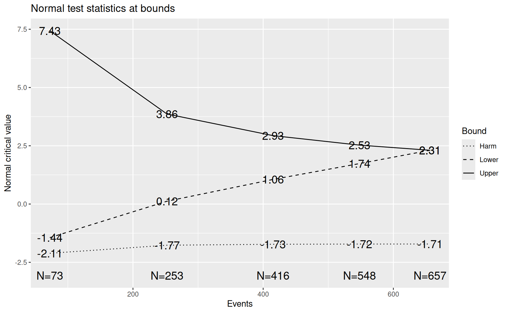

Figure 15.1: Z-value boundaries for non-binding harm bound design

plot(x8, plottype = 2)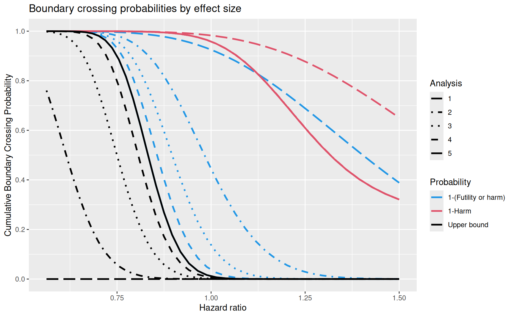

Figure 15.2: Boundary crossing probabilities for non-binding harm bound design

plot(x8, plottype = 3)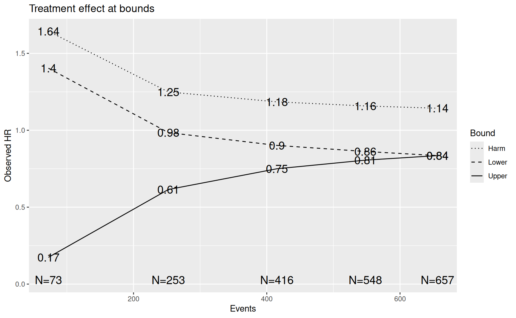

Figure 15.3: Approximate treatment effect at boundaries

plot(x8, plottype = 5)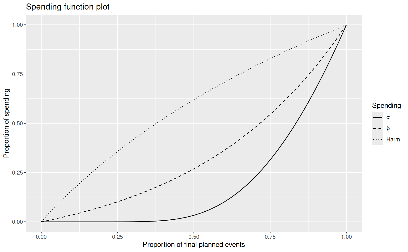

Figure 15.4: Spending functions for non-binding harm bound design

plot(x8, plottype = 7)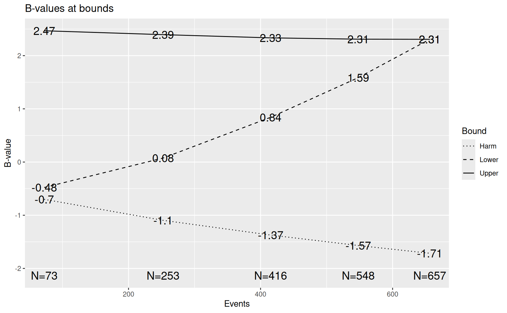

15.3 Design with binding bounds (`test.type = 7`)

For test.type = 7, both the futility and harm bounds are binding — meaning the computation of the efficacy bound assumes the trial will stop if either bound is crossed. This yields a slightly less conservative efficacy bound, but at the cost of inflated Type I error if the stopping rule is not strictly followed.

x7 <- gsSurvCalendar(
  test.type = 7,
  alpha = 0.0125,
  beta = 0.1,
  astar = 0.1,
  calendarTime = c(12, 24, 36, 48, 60),
  sfu = sfLDOF,
  sfl = sfHSD, sflpar = -2,
  sfharm = sfLDPocock,
  lambdaC = log(2) / 36,
  hr = 0.75,
  R = 18,
  minfup = 42
)

15.3.1 Comparing binding and non-binding

comparison <- data.frame(
  Bound = c("Efficacy", "Futility", "Harm"),
  `Binding (type 7)` = c(
    paste(round(x7$upper$bound, 3), collapse = ", "),
    paste(round(x7$lower$bound, 3), collapse = ", "),
    paste(round(x7$harm$bound, 3), collapse = ", ")
  ),
  `Non-binding (type 8)` = c(
    paste(round(x8$upper$bound, 3), collapse = ", "),
    paste(round(x8$lower$bound, 3), collapse = ", "),
    paste(round(x8$harm$bound, 3), collapse = ", ")
  ),
  check.names = FALSE
)
knitr::kable(comparison,
  caption = "Comparison of binding vs. non-binding Z-value boundaries"
)

Comparison of binding vs. non-binding Z-value boundaries
Bound	Binding (type 7)	Non-binding (type 8)
Efficacy	7.434, 3.862, 2.934, 2.523, 2.248	7.434, 3.862, 2.935, 2.528, 2.307
Futility	-1.458, 0.09, 1.016, 1.689, 2.248	-1.441, 0.121, 1.057, 1.736, 2.307
Harm	-2.112, -1.767, -1.726, -1.717, -1.715	-2.112, -1.767, -1.726, -1.717, -1.715

The efficacy bounds for test.type = 7 are slightly lower (easier to cross) than for test.type = 8. The maximum number of events for test.type = 7 (639) is also slightly smaller than for test.type = 8 (657).

gsBoundSummary(x7)
#> Method: LachinFoulkes 
#>     Analysis               Value    Harm Futility Efficacy
#>    IA 1: 11%                   Z -2.1121  -1.4578       NA
#>       N: 746         p (1-sided)  0.9827   0.9275       NA
#>   Events: 71        ~HR at bound  1.6550   1.4158       NA
#>    Month: 12    P(Cross) if HR=1  0.0173   0.0551       NA
#>              P(Cross) if HR=0.75  0.0005   0.0034       NA
#>    IA 2: 38%                   Z -1.7667   0.0895   3.8622
#>      N: 1118         p (1-sided)  0.9614   0.4643   0.0001
#>  Events: 246        ~HR at bound  1.2531   0.9886   0.6107
#>    Month: 24    P(Cross) if HR=1  0.0419   0.5011   0.0001
#>              P(Cross) if HR=0.75  0.0005   0.0176   0.0539
#>    IA 3: 63%                   Z -1.7256   1.0159   2.9344
#>      N: 1118         p (1-sided)  0.9578   0.1548   0.0017
#>  Events: 404        ~HR at bound  1.1874   0.9038   0.7467
#>    Month: 36    P(Cross) if HR=1  0.0421   0.8131   0.0017
#>              P(Cross) if HR=0.75  0.0005   0.0393   0.4829
#>    IA 4: 83%                   Z -1.7170   1.6890   2.5229
#>      N: 1118         p (1-sided)  0.9570   0.0456   0.0058
#>  Events: 533        ~HR at bound  1.1604   0.8639   0.8037
#>    Month: 48    P(Cross) if HR=1  0.0421   0.9172   0.0063
#>              P(Cross) if HR=0.75  0.0005   0.0670   0.7881
#>        Final                   Z -1.7149   2.2480   2.2480
#>      N: 1118         p (1-sided)  0.9568   0.0123   0.0123
#>  Events: 639        ~HR at bound  1.1454   0.8370   0.8370
#>    Month: 60    P(Cross) if HR=1  0.0421   0.9455   0.0125
#>              P(Cross) if HR=0.75  0.0005   0.0995   0.9000

15.3.2 Efficacy bounds at alternate \(\alpha\) levels

The gsBoundSummary() function accepts an alpha argument to display efficacy bounds at alternate \(\alpha\) levels alongside the original design:

gsBoundSummary(x8, alpha = 0.025)
#>     Analysis               Value α=0.0125 α=0.025 Futility
#>    IA 1: 11%                   Z       NA      NA  -1.4408
#>       N: 766         p (1-sided)       NA      NA   0.9252
#>   Events: 73        ~HR at bound       NA      NA   1.4034
#>    Month: 12    P(Cross) if HR=1       NA      NA   0.0575
#>              P(Cross) if HR=0.75       NA      NA   0.0034
#>    IA 2: 38%                   Z   3.8622  3.4312   0.1212
#>      N: 1148         p (1-sided)   0.0001  0.0003   0.4518
#>  Events: 253        ~HR at bound   0.6149  0.6492   0.9849
#>    Month: 24    P(Cross) if HR=1   0.0001  0.0003   0.5138
#>              P(Cross) if HR=0.75   0.0574  0.1259   0.0177
#>    IA 3: 63%                   Z   2.9347  2.5948   1.0566
#>      N: 1148         p (1-sided)   0.0017  0.0047   0.1454
#>  Events: 416        ~HR at bound   0.7497  0.7751   0.9015
#>    Month: 36    P(Cross) if HR=1   0.0017  0.0048   0.8224
#>              P(Cross) if HR=0.75   0.4990  0.6323   0.0394
#>    IA 4: 83%                   Z   2.5278  2.2359   1.7357
#>      N: 1148         p (1-sided)   0.0057  0.0127   0.0413
#>  Events: 548        ~HR at bound   0.8057  0.8261   0.8622
#>    Month: 48    P(Cross) if HR=1   0.0062  0.0138   0.9214
#>              P(Cross) if HR=0.75   0.7996  0.8684   0.0670
#>        Final                   Z   2.3072  2.0432   2.3072
#>      N: 1148         p (1-sided)   0.0105  0.0205   0.0105
#>  Events: 657        ~HR at bound   0.8352  0.8526   0.8352
#>    Month: 60    P(Cross) if HR=1   0.0112  0.0201   0.9471
#>              P(Cross) if HR=0.75   0.9000  0.9218   0.0996
#>     Harm
#>  -2.1121
#>   0.9827
#>   1.6434
#>   0.0173
#>   0.0004
#>  -1.7667
#>   0.9614
#>   1.2491
#>   0.0416
#>   0.0004
#>  -1.7256
#>   0.9578
#>   1.1846
#>   0.0417
#>   0.0004
#>  -1.7170
#>   0.9570
#>   1.1580
#>   0.0417
#>   0.0004
#>  -1.7149
#>   0.9568
#>   1.1433
#>   0.0417
#>   0.0004

15.4 Practical considerations

15.4.1 Choice of spending functions

Efficacy: A conservative spending function such as Lan-DeMets O’Brien-Fleming (sfLDOF) is typical.
Futility: Moderate spending (e.g., HSD with \(\gamma = -2\)) allows early stopping for futility.
Harm: Lan-DeMets Pocock (sfLDPocock) provides more aggressive spending at early analyses, appropriate for harm monitoring since detecting a detrimental effect early is critical for patient safety.

15.4.2 Interpreting the harm bound

The harm bound is intended so that if a small observed \(p\)-value favoring control is observed, the harm bound will be crossed. A negative Z-value indicates that the hazard rate is higher in the experimental arm — the experimental treatment appears to be worsening survival. When the Z-value falls below the harm bound, this constitutes a statistical signal that the treatment may be harmful.

The harm spending is computed under \(H_0\) (no treatment effect), controlling the probability of a false harm signal.

15.4.3 Harm bound capping

The harm bound is automatically capped so it never exceeds the futility bound, ensuring the ordering: harm bound \(\leq\) futility bound \(\leq\) efficacy bound at every analysis.

15.4.4 When to use `test.type = 7` vs. `test.type = 8`

test.type = 8 (non-binding) is most often preferred in practice. It preserves Type I error control regardless of whether the stopping rules are strictly followed. Since Data Monitoring Committees typically retain discretion to continue or stop a trial, the non-binding approach ensures statistical validity.
test.type = 7 (binding) provides a small efficiency gain but requires strict protocol adherence. If the trial does not stop after crossing a binding boundary, Type I error may be inflated.

15.5 Selective bound testing

In many clinical trial designs, it is desirable to test only certain boundaries at specific interim analyses. The testUpper, testLower, and testHarm parameters in gsDesign(), gsSurv(), and gsSurvCalendar() allow fine-grained control over which bounds are active at each analysis. When a bound is inactive, it is set to an extreme value (\(\pm 20\) on the Z-scale) and displayed as NA in summaries.

15.5.1 Example: Futility testing only at the first interim

A common scenario is to test for futility only at the first interim analysis.

x1 <- gsDesign(
  k = 3,
  test.type = 4,
  alpha = 0.025,
  beta = 0.1,
  sfu = sfHSD, sfupar = -4,
  sfl = sfHSD, sflpar = -2,
  testLower = c(TRUE, FALSE, FALSE)
)
gsBoundSummary(x1)
#>                Analysis               Value Efficacy Futility
#>               IA 1: 33%                   Z   3.0107  -0.2674
#>  N/Fixed design N: 0.35         p (1-sided)   0.0013   0.6054
#>                             ~delta at bound   1.5787  -0.1402
#>                         P(Cross) if delta=0   0.0013   0.3946
#>                         P(Cross) if delta=1   0.1349   0.0148
#>               IA 2: 67%                   Z   2.5465       NA
#>  N/Fixed design N: 0.69         p (1-sided)   0.0054       NA
#>                             ~delta at bound   0.9442       NA
#>                         P(Cross) if delta=0   0.0062       NA
#>                         P(Cross) if delta=1   0.5657       NA
#>                   Final                   Z   1.9992       NA
#>  N/Fixed design N: 1.04         p (1-sided)   0.0228       NA
#>                             ~delta at bound   0.6052       NA
#>                         P(Cross) if delta=0   0.0244       NA
#>                         P(Cross) if delta=1   0.9000       NA

The lower bound is active only at IA1. At IA2 and the final analysis, the futility bound shows as NA.

plot(x1, plottype = 1)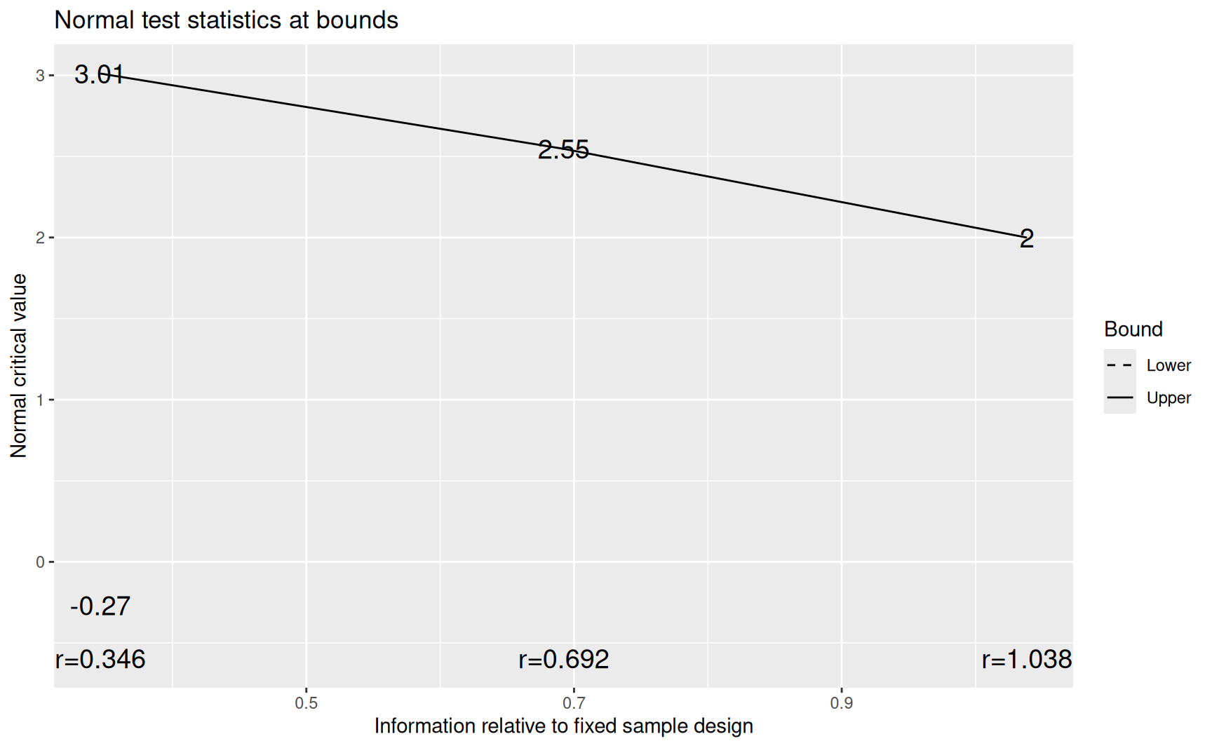

Figure 15.6: Bounds with futility only at IA1

15.5.2 Example: No efficacy testing at the first interim

Efficacy testing may be deferred until sufficient data have accrued:

x2 <- gsDesign(
  k = 3,
  test.type = 3,
  alpha = 0.025,
  beta = 0.1,
  sfu = sfHSD, sfupar = -4,
  sfl = sfHSD, sflpar = -2,
  testUpper = c(FALSE, TRUE, TRUE)
)
gsBoundSummary(x2)
#>                Analysis               Value Efficacy Futility
#>               IA 1: 33%                   Z       NA  -0.2605
#>  N/Fixed design N: 0.35         p (1-sided)       NA   0.6028
#>                             ~delta at bound       NA  -0.1361
#>                         P(Cross) if delta=0       NA   0.3972
#>                         P(Cross) if delta=1       NA   0.0148
#>               IA 2: 67%                   Z   2.4976   0.9102
#>   N/Fixed design N: 0.7         p (1-sided)   0.0063   0.1814
#>                             ~delta at bound   0.9227   0.3363
#>                         P(Cross) if delta=0   0.0062   0.8270
#>                         P(Cross) if delta=1   0.5826   0.0437
#>                   Final                   Z   1.9597   1.9597
#>  N/Fixed design N: 1.05         p (1-sided)   0.0250   0.0250
#>                             ~delta at bound   0.5911   0.5911
#>                         P(Cross) if delta=0   0.0250   0.9750
#>                         P(Cross) if delta=1   0.9000   0.1000

15.5.3 Example: Selective harm monitoring

For designs with a harm bound, testHarm controls which analyses include harm monitoring:

xh <- gsDesign(
  k = 3,
  test.type = 8,
  alpha = 0.025,
  beta = 0.1,
  astar = 0.05,
  sfu = sfHSD, sfupar = -4,
  sfl = sfHSD, sflpar = -2,
  sfharm = sfHSD, sfharmparam = 1,
  testHarm = c(TRUE, TRUE, FALSE)
)
gsBoundSummary(xh)
#>                Analysis               Value    Harm Futility
#>               IA 1: 33%                   Z -2.0061  -0.2387
#>  N/Fixed design N: 0.36         p (1-sided)  0.9776   0.5943
#>                             ~delta at bound -1.0363  -0.1233
#>                         P(Cross) if delta=0  0.0224   0.3832
#>                         P(Cross) if delta=1  0.0000   0.0148
#>               IA 2: 67%                   Z -1.9827   0.9411
#>  N/Fixed design N: 0.71         p (1-sided)  0.9763   0.1733
#>                             ~delta at bound -0.7242   0.3438
#>                         P(Cross) if delta=0  0.0231   0.8116
#>                         P(Cross) if delta=1  0.0000   0.0437
#>                   Final                   Z      NA   1.9992
#>  N/Fixed design N: 1.07         p (1-sided)      NA   0.0228
#>                             ~delta at bound      NA   0.5963
#>                         P(Cross) if delta=0      NA   0.9536
#>                         P(Cross) if delta=1      NA   0.1000
#>  Efficacy
#>    3.0107
#>    0.0013
#>    1.5553
#>    0.0013
#>    0.1412
#>    2.5465
#>    0.0054
#>    0.9302
#>    0.0062
#>    0.5815
#>    1.9992
#>    0.0228
#>    0.5963
#>    0.0233
#>    0.9000

15.5.4 Validation rules

The following rules are enforced:

testUpper must be TRUE at the final analysis.
At least one bound must be active at every analysis.
For test.type 3–8, testLower must be TRUE for at least one analysis.
For test.type 7 and 8, testHarm must be TRUE for at least one analysis.

15.5.5 Type I error preservation

When bounds are selectively deactivated, Type I error is preserved at the nominal level. At inactive analyses, the cumulative spending is frozen. At the next active analysis, the incremental spend absorbs the budget from skipped analyses, so the cumulative spend catches up to the planned level.

# Baseline non-binding design
x_nb <- gsDesign(k = 3, test.type = 4, alpha = 0.025, beta = 0.1)

# Remove futility at IA2 and final
x_nb_sel <- gsDesign(
  k = 3, test.type = 4, alpha = 0.025, beta = 0.1,
  testLower = c(TRUE, FALSE, FALSE)
)

# Verify upper bounds are identical (non-binding case)
cat(
  "Upper bounds identical:",
  all.equal(x_nb$upper$bound, x_nb_sel$upper$bound),
  "\n"
)
#> Upper bounds identical: TRUE